Incorporating
Grid-based Terrain Modeling
into Linear
Infrastructure Analysis
Joseph K. Berry
Senior Consultant, New Century Software
Keck Scholar in Geosciences,
Principal, Berry & Associates // Spatial
Information Systems
Email: jberry@innovativegis.com — Website: www.innovativegis.com/basis/
Nate Mattie
Email: natem@newcenturysoftware.com —
Website: www.newcenturysoftware.com
<Paper presented at GITA
Conference,
<Click
here> for a printer-friendly version (.pdf)
ABSTRACT
Grid-based map analysis is increasingly used to characterize conditions and impacts of infrastructure networks, such as pipe and power lines. “Off-line” concerns are driving new regulations for assessing potential impacts and consequences, as well as new demands by corporations for better portrayals of conditions along a linear asset. Terrain-modeling includes a variety of procedures for assessing surface configuration and flows that address these concerns. This paper describes the application of several techniques for determining micro-terrain characteristics (slope/aspect and surface inflection), elevation profile segmentation and characterization and overland flow modeling of spill migration. Particular attention is devoted to the interactions between discrete (vector) and continuous (raster) systems. Discussion is extended to considerations in the practical application of these techniques through several case studies.
Introduction
Linear infrastructure applications using Geographic
Information Systems (
These differences go well beyond the technical aspects of geo-referencing; they identify differences in perspective of applications and business models defining the utility of geo-processing. The “stationing” approach is focused on the linear asset itself, while the “vector” broadens the focus to other point, line and polygon features surrounding a route. However, both approaches treat geographic space as composed of set of discrete spatial objects analogous to puzzle pieces defining a project area.
“Raster” systems, on the other hand, treat geographic space as a continuum and extend point, line and polygon features to map surfaces. These gradients characterize the spatial distributions of continuous phenomena that continually change throughout geographic space. In addition, this grid-based structure expresses mapped data in a numerical context that supports an extensive set of mathematical and statistical operations for analyzing relationships within and among mapped data layers.
Most contemporary infrastructure software packages have fully integrated the stationing and vector approaches. This bundling provides a wide array of operations for geo-query of spatial databases and mapping the results. In addition, raster images can be geo-registered and used as a backdrop for display resulting in extremely useful systems for constructing, maintaining and querying infrastructure data.
However, applications involving grid-based analysis “off the
lines” are less familiar to
Understanding Grid-based Data
For thousands of years, points, lines and polygons have been used to depict map features. With the stroke of a pen a cartographer could outline a continent, delineate a highway or identify a specific building’s location. With the advent of the computer, manual drafting of these data has been replaced by the cold steel of the plotter.
In digital form these spatial data have been linked to attribute tables that describe characteristics and conditions of the map features. Desktop mapping exploits this linkage to provide tremendously useful database management procedures, such as address matching, geo-query and routing. Vector-based data forms the foundation of these techniques and directly builds on our historical perspective of maps and map analysis.
Grid-based data, on the other hand, is a relatively new way to describe geographic space and its relationships. Weather maps, identifying temperature and barometric pressure gradients, were an early application of this new data form. In the 1950s computers began analyzing weather station data to automatically draft maps of areas of specific temperature and pressure conditions. At the heart of this procedure is a new map feature that extends traditional points, lines and polygons (discrete objects) to continuous surfaces.
Figure 1 outlines the major differences between discrete and continuous mapped data. Discrete maps identify mapped data with independent numbers forming sharp abrupt boundaries, such as a Covertype map. Continuous maps, on the other hand, contain a range of values that form spatial gradients, such as an Elevation surface.

Figure 1. Visualizing the differences
between discrete and continuous representations of mapped data.
Note that the 3D display of a Covertype map as a surface is inappropriate as the map values (1= water, 2= meadow and 3= forest) have no numerical relationship with one another and that each feature has a sharp boundary. A surface view of the Elevation map, however, is appropriate as the data is constantly changing. Its 2D contour display is inappropriate as it generalizes the spatial variability into a few broad classes forming polygons that contain a wide range of individual elevation values.
Forcing a continuous spatial variable (surface) into its vector-based representation oversimplifies the spatial pattern and severely limits further analytical processing. The following examples of surface analysis focuses on characterizing terrain conditions and flows as applied in contemporary pipeline industry applications.
Micro-Terrain Characteristics
A terrain surface is
organized as a rectangular "analysis grid" with each cell containing
an elevation value. The upper-left inset
in Figure 2 shows a smoothed lattice-display of the elevation surface with its
2D contour lines projected onto the floor of the 3D plot. The larger plot is a grid-display each
cell to the relative height of its
elevation value.
There are several
roving window operations that track the spatial arrangement of the elevation
values as well as aggregate statistics.
A frequently used one is terrain slope that calculates the
"slant" of a surface. In
mathematical terms, slope equals the difference in elevation (termed the
"rise") divided by the horizontal distance (termed the
"run").
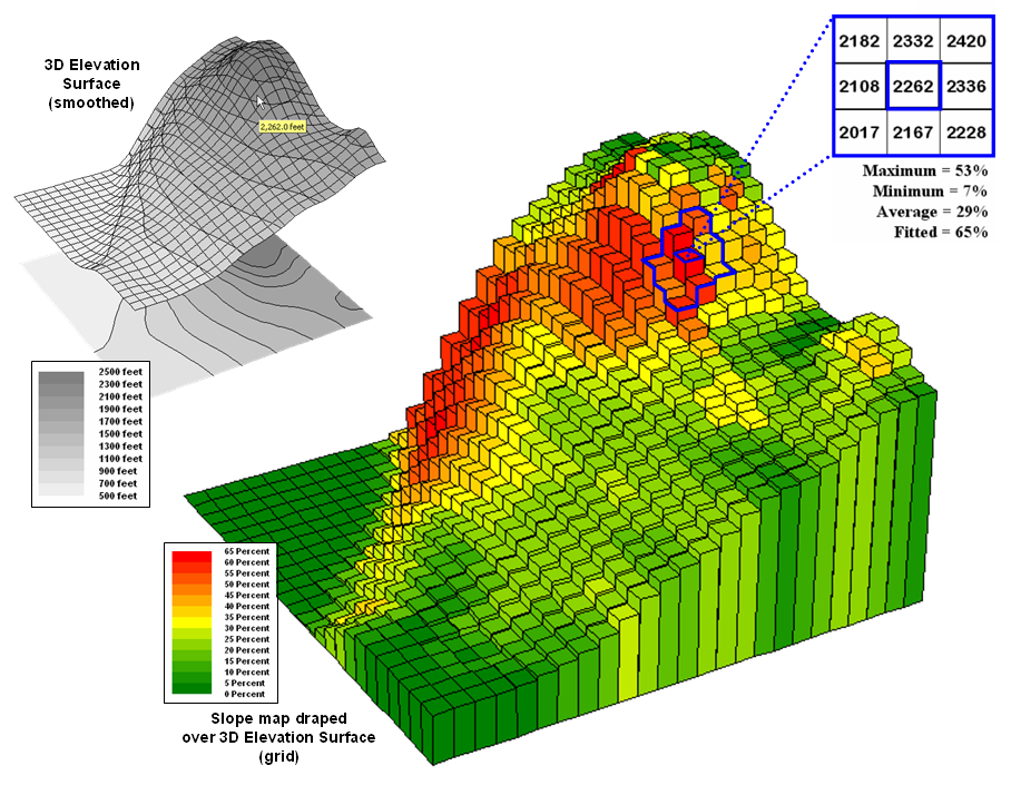
Figure 2. Elevation surface with its slope map graphically overlaid.
In calculating slope, a 3x3 window is used to identify elevation values
surrounding an individual grid location as shown on the left side of figure
2. An individual slope value from the
center cell can be calculated for each one of the eight adjacent cells. For example, the percent slope to the north
(top of the window) is ((2332 - 2262) / 328) * 100 = 21.3%. The numerator computes the rise while the denominator
of 328 feet is the distance between the centers of the two cells. The calculations for the northeast slope is
((2420 - 2262) / 464) * 100 = 34.1%, where the run is increased to account for
the diagonal distance (328 * 1.414 = 464).
Note that the sign of the eight individual slope values indicates the direction
of surface flow—positive slopes indicate flows into the center cell while
negative ones indicate flows out. While
the flow into the center cell depends on the uphill conditions (to be discussed
in the last section on overland flow), the flow away from the cell will take
the steepest downhill slope—southwest flow in the example.
The eight slope values can be used to identify the Maximum and Minimum
slope as reported in the figure. Note
that the large difference between the maximum and minimum slope values (53 - 7
= 46) suggests that the overall slope around the center cell is fairly
variable.
In addition, the eight individual slopes can be used to calculate
transverse and longitudinal slope for locations along a linear feature, such as
a proposed pipeline route. In this
instance, the 3x3 window moves along the cells defining the route and
separately averages the individual slopes containing the route (longitudinal)
and those outside the route (transverse).
An estimate of the overall slope for a location is derived by averaging
all eight individual slopes. However,
the simple Average can be misleading. It
is supposed to indicate the overall slant within the window but fails to account
for the spatial arrangement of the slope values. An alternative technique fits a “plane” to
the nine individual elevation values.
The procedure determines the best fitting plane by minimizing the
deviations from the plane to the elevation values. In the example, the Fitted slope value is
65%—more than the maximum individual slope.
The 3D grid plot in Figure 2 shows the results derived by "fitting
a plane" to the nine elevation values surrounding each map location. Note that larger slope values (reds) align
with the steeper areas of the surface, while lower values (greens) align with
gentle slopes and flat areas.
The use of a fitted plane for
calculations also provides a procedure for calculating aspect (directional
orientation at each cell location comprising the surface). The technique uses a bit trigonometry by
calculating the “direction cosines” of the fitted plane to identify its
orientation as an azimuth value between 0 (north) and 360. For the example location, the azimuth is 221
degrees (SW bearing).
Elevation Profile Segmentation
Slope is a critical factor in both siting and operating a pipeline. In general, crossing areas of steep slopes are avoided whenever possible when designing new routes. Once a proposed route has been identified slope plays a dominant role in determining the location of compressor facilities along the route.
It is imperative that a meaningful terrain profile is generated. The line segments defining the profile cannot contain elevation values that are significantly higher or lower than the end points or the calculated slope length will be too inaccurate for determining compressor location.
Neither “stationing” nor “vector-based” approaches are aware of the full continuum of elevation values throughout a project area. A “raster-based” system, on the other hand, is fully aware of subtle elevation differences for identifying the peaks and valleys in an elevation surface.
Figure 3 outlines a frequently used technique that involves subtracting a “smoothed elevation” value from
the actual elevation value at a given location.
A window is used to average the elevations over a several-cell reach in
both directions of a route location under consideration. This has the effect of “smoothing” the
elevation to its trend line. Subtracting
the trend value from the actual elevation determines the type and magnitude of
a terrain deflection —positive difference values indicate “convex features”
protruding above the surface’s trend line; negative values indicate “concave
features.” The magnitude of the
difference indicates the relative height (or depth) of the micro terrain
feature.

Figure 3. Identifying Convex and Concave features by deviation from the terrain’s trend.
In segmenting the terrain along a proposed route, a change in sign indicates an inflection point that can be used as an end point for terrain segments. If the change in sign isn’t significant (small value) then a break is not warranted. The schematic at the bottom of figure 3 illustrates the variable length of segments defined by coincidence of a proposed route with major inflection points along an elevation surface.
Overland Flow Modeling
Now consider a far more complex terrain analysis problem. The pipeline industry has been mandated to determine the flows that would occur if a release were to happen at any location along a pipeline route. Figure 4 outlines the major steps of an “Overland Flow” model that tracks potential spill migration. The first step positions a pipeline on an elevation surface. Then a spill point along the pipeline is identified and its overland flow path (downhill) identified. In an iterative fashion, successive spill points and their paths are identified.
High Consequence Areas (HCAs) are delineated on maps prepared by the Office of Pipeline Safety. These include areas such as high population concentrations, drinking water supplies and critical ecological zones. The HCAs impacted by individual spills are identified and recorded in a database table. The final step identifies where paths enter streams or lakes and passes the information to a Channel Flow module.
Developing a realistic model of overland flow is complex and needs to consider differences in terrain slopes, product types and intervening conditions. In addition, information on the timing and quantity of flow as the path progresses is invaluable in spill migration planning.
At the heart of the solution is the ability to identify path flow. As mentioned in the previous discussion on calculating slope, the sign of the eight individual slopes surrounding a grid location on an elevation surface identifies the direction of flow with negative values indicating flows away from the center cell. The magnitude of the slope value indicates how steep the step is.

Figure 4. Spill mitigation for pipelines identifies high consequence areas that could be impacted if a spill occurs anywhere along a pipeline.
Figure 5 illustrates two downhill paths over a terrain surface. A starting point on the surface is identified and the computer simulates the downhill route by selecting “the steepest downhill path” at each step along the grid surface.
As shown in the enlarged inset on the right side of the figure, a location along the path could potentially flow to any of its neighboring cells. Uphill possibilities with larger elevation values are immediately eliminated. The steepest downhill step is determined and path flow moves to that location. The process is repeated over and over to identify the steps along the steepest downhill path.
This procedure works nicely until reality sets in. What happens when a flat area is encountered? No longer is there a single steepest downhill step because all surrounding elevation values are equal or larger. Obviously the flow doesn’t stop; it simply spreads out into the flat area. In this instance the algorithm must incorporate code that continues spreading as shown in the figure. The “steepest downhill path, then stop at flat areas” approach is not sufficient. Nor is a path that simply shoots a straight line across a flat area a realistic solution.

Figure 5. Surface flow takes the
steepest downhill path whenever possible but spreads out in flat areas and
pools in depressions.
However, realistic flow modeling is even more subtle than that. Areas of very gentle slope but not perfectly flat tend to exhibit sheet flow and spread out to all of the slight downhill locations. Figure 6 depicts the different conditions for path, sheet and flat flow.

Figure 6. Surface inclination and liquid type determine the type of surface flow—path, sheet or flat.
Incorporating sheet flow into the algorithm inserts a test that determines if the steepest downhill step is less than a specified angle—if so, then steps to all of the downhill locations are taken. Another confounding condition occurs when there are equally steep downhill possibilities. In this instance both steps are taken and the flow path broadens or splits.
By far the trickiest flow for a computer to simulate is pooling. Figure 7 shows a path that seemingly stops when it reaches a depression. In this instance, all of the elevation values around it are larger and there are no downhill or across steps to take. As flow continues the depression fills. When the quantity reaches the height of the smallest elevation surrounding the depression the flow moves into it.

Figure 7. Pooling of surface
flow occurs when depressions are encountered.
This is the same procedure the computer algorithm uses. It searches the neighboring cells for the smallest elevation, fills to that level, and then steps to that location. The procedure of filling and stepping is repeated until the lip of the depression is breached and downhill flow can resume.
Another possibility is that the quantity of flowing liquid
is exhausted and the path terminated at a pooling depth that fails to
completely fill the depression. The idea
of tracking flow quantity, as well as elapsed time, along a flow path is an
important one, particularly when modeling pipeline spill migration. If a stream
channel is encountered, the spill quantity and timing for the entry point is
automatically transferred to a vector-based channel flow module and continues
along the stream network for a specified distance or time.
Figure 8 shows real-world results from the Spill Migration
AnalystTM module to ArcGIS by New Century Software,
Incorporated. The user supplies
information about pipeline characteristics, product type and spill simulation
locations or spacing. The software moves
along the pipeline stopping at a specified location and then generates a
simulated overland spill path and channel flow if a stream is encountered. The primary
map out is an alignment sheet identifying the

Figure 8. Example output from
Spill Migration AnalystTM.
The spill migration output
can be integrated into an alignment sheet format identifying the
Conclusion
Grid-based map analysis procedures provide a wealth of
capabilities for incorporating terrain information surrounding linear
infrastructure. Although the procedures described have important practical
applications, a hidden agenda of the discussions was to get readers to think of
geographic space in a less traditional way—as an organized set of numbers
(numerical data), instead of points, lines and areas represented by various
colors and patterns (graphic map features).
Online References
See the online book Map
Analysis by Joseph K. Berry (BASIS Press) that is posted at
www.innovativegis.com/basis
Select the following
topics for more information on grid-based map analysis and procedures for
analyzing terrain conditions and flows (listed in order of discussion this
paper):
¾
Topic 18,
Understanding Grid-based Data
¾
Topic 11,
Characterizing Micro Terrain Features
¾
Topic 20, Surface
Flow Modeling
¾
Topic 19, Routing
and Optimal Paths
_______________________
Paper with full color figures
is posted online at www.innovativegis.com/basis/Present/GITA_Denver05/