Beyond Mapping III
|
Map
Analysis book with companion CD-ROM
for hands-on exercises and further reading |
Early GIS Technology and Its Expression — traces
the early phases of GIS technology (Computer Mapping, Spatial Database
Management and Map Analysis/Modeling)
Contemporary GIS and Future Directions — discusses
contemporary GIS and probable future directions (Multimedia Mapping and Spatial
Reasoning/Dialog)
Pathways
to GIS — explores different paths of GIS adoption for five disciplines
(Natural Resources, Facilities Management, Public Health, Business and
Precision Agriculture)
A Multifaceted GIS Community — investigates
the technical shifts and cultural impacts of the rapidly expanding GIS tent of
users, application developers and tool programmers
Innovation Drives GIS Evolution — discusses the
cyclic nature of GIS innovation (Mapping, Structure and Analysis)
GIS and the Cloud Computing Conundrum — describes cloud computing with particular
attention to its geotechnology expression
Visualizing a Three-dimensional Reality
— uses visual connectivity to introduce and reinforce the paradigm of
three-dimension geography
Thinking Outside the Box — discusses
concepts and configuration of 3-dimensional geography
From
a Map Pancake to Soufflé — continues the discussion of concepts and
configuration of a 3D GIS
Note: The processing and figures
discussed in this topic were derived using MapCalcTM software.
See www.innovativegis.com to download
a free MapCalc Learner version with tutorial materials for classroom and
self-learning map analysis concepts and procedures.
<Click here>
right-click to download a printer-friendly version of this topic (.pdf).
(Back to the Table of Contents)
______________________________
Early GIS
Technology and Its Expression
(GeoWorld October, 2006)
Considerable
changes in both expectations and capabilities have taken place since GIS’s
birth in the late 1960s. In this and a
few subsequent columns, I hope to share a brief history and a probable future
of this rapidly maturing field as viewed from grey-beard experience from over
30 years involvement in the field (see Author’s Note).
Overview
Information has always been the cornerstone of effective decisions. Spatial information is particularly complex
as it requires two descriptors—Where is What. For thousands of years the link between the
two descriptors has been the traditional, manually drafted map involving pens,
rub-on shading, rulers, planimeters, dot grids, and acetate sheets. Its historical use was for navigation through
unfamiliar terrain and seas, emphasizing the accurate location of physical
features.
More recently, analysis of mapped data has become an important part of
understanding and managing geographic space.
This new perspective marks a turning point in the use of maps from one emphasizing
physical description of geographic space, to one of interpreting mapped data,
combining map layers and finally, to spatially characterizing and communicating
complex spatial relationships. This
movement from “where is what” (descriptive) to "so what and why"
(prescriptive) has set the stage for entirely new geospatial concepts and
tools.
Since
the 1960's, the decision-making process has become increasingly quantitative,
and mathematical models have become commonplace. Prior to the computerized map, most spatial
analyses were severely limited by their manual processing procedures. The computer has provided the means for both
efficient handling of voluminous data and effective spatial analysis capabilities. From this perspective, all geographic
information systems are rooted in the digital nature of the computerized map.
The coining of the term Geographic Information Systems reinforces this movement
from maps as images to mapped data. In
fact, information is GIS's middle name.
Of course, there have been other, more descriptive definitions of the
acronym, such as "Gee It's Stupid," or "Guessing Is
Simpler," or my personal favorite, "Guaranteed Income Stream."
Computer Mapping (1970s, Beginning
Years)
The early 1970's saw computer mapping automate map drafting. The points,
lines and areas defining geographic features on a map are represented as an
organized set of X, Y coordinates. These data drive pen plotters that can
rapidly redraw the connections at a variety of colors, scales, and projections
with the map image, itself, as the focus of the processing.
The
pioneering work during this period established many of the underlying concepts
and procedures of modern GIS technology. An obvious advantage with computer
mapping is the ability to change a portion of a map and quickly redraft the
entire area. Updates to resource maps which could take weeks, such as a forest
fire burn, can be done in a few hours. The less obvious advantage is the
radical change in the format of mapped data— from analog inked lines on paper,
to digital values stored on disk.
Spatial Database Management (1980s,
Adolescent Years)
During 1980's, the change in data format and computer environment was
exploited. Spatial database management systems were developed that
linked computer mapping capabilities with traditional database management
capabilities. In these systems,
identification numbers are assigned to each geographic feature, such as a
timber harvest unit or ownership parcel.
For example, a user is able to point to any location on a map and
instantly retrieve information about that location. Alternatively, a user can specify a set of
conditions, such as a specific forest and soil combination, then direct the
results of the geographic search to be displayed as a map.
Early
in the development of GIS, two alternative data structures for encoding maps
were debated. The vector data model closely mimics
the manual drafting process by representing map features (discrete spatial objects)
as a set of lines which, in turn, are stores as a series of X,Y
coordinates. An alternative structure,
termed the raster data model,
establishes an imaginary grid over a project area, and then stores resource
information for each cell in the grid (continuous map surface). The early debate attempted to determine the
universally best structure. The relative
advantages and disadvantages of both were viewed in a competitive manner that
failed to recognize the overall strengths of a GIS approach encompassing both
formats.
By the
mid-1980's, the general consensus within the GIS community was that the nature
of the data and the processing desired determines the appropriate data
structure. This realization of the
duality of mapped data structure had significant impact on geographic
information systems. From one
perspective, maps form sharp boundaries that are best represented as
lines. Property ownership, timber sale
boundaries, and road networks are examples where lines are real and the data
are certain. Other maps, such as soils,
site index, and slope are interpretations of terrain conditions. The placement of lines identifying these
conditions is subject to judgment and broad classification of continuous
spatial distributions. From this
perspective, a sharp boundary implied by a line is artificial and the data
itself is based on probability.
Increasing
demands for mapped data focused attention on data availability, accuracy and
standards, as well as data structure issues.
Hardware vendors continued to improve digitizing equipment, with manual
digitizing tablets giving way to automated scanners at many GIS
facilities. A new industry for map
encoding and database design emerged, as well as a marketplace for the sales of
digital map products. Regional, national
and international organizations began addressing the necessary standards for
digital maps to insure compatibility among systems. This era saw GIS database development move
from project costing to equity investment justification in the development of
corporate databases.
Map Analysis and Modeling (1990s,
Maturing Years)
As GIS continued its evolution, the emphasis turned from descriptive query to
prescriptive analysis of maps. If early
GIS users had to repeatedly overlay several maps on a light-table, an analogous
procedure was developed within the GIS.
Similarly, if repeated distance and bearing calculations were needed,
the GIS system was programmed with a mathematical solution. The result of this effort was GIS
functionality that mimicked the manual procedures in a user's daily
activities. The value of these systems
was the savings gained by automating tedious and repetitive operations.
By the
mid-1980's, the bulk of descriptive query operations were available in most GIS
systems and attention turned to a comprehensive theory of map analysis. The dominant feature of this theory is that
spatial information is represented numerically, rather than in analog fashion
as inked lines on a map. These digital
maps are frequently conceptualized as a set of "floating maps" with a
common registration, allowing the computer to "look" down and across
the stack of digital maps. The spatial
relationships of the data can be summarized (database queries) or
mathematically manipulated (analytic processing). Because of the analog nature of traditional
map sheets, manual analytic techniques are limited in their quantitative
processing. Digital representation, on
the other hand, makes a wealth of quantitative (as well as qualitative)
processing possible. The application of
this new theory to mapping was revolutionary and its application takes two
forms—spatial statistics and spatial analysis.
Meteorologists
and geophysicists have used spatial
statistics for decades to characterize the geographic distribution,
or pattern, of mapped data. The
statistics describe the spatial variation in the data, rather than assuming a
typical response is everywhere. For
example, field measurements of snow depth can be made at several plots within a
watershed. Traditionally, these data are
analyzed for a single value (the average depth) to characterize an entire
watershed. Spatial statistics, on the
other hand, uses both the location and the measurements at sample locations to
generate a map of relative snow depth throughout the watershed. This numeric-based processing is a direct
extension of traditional non-spatial statistics.
Spatial analysis applications, on the other hand, involve
context-based processing. For example,
forester’s can characterize timber supply by considering the relative skidding
and log-hauling accessibility of harvesting parcels. Wildlife managers can
consider such factors as proximity to roads and relative housing density to map
human activity and incorporate this information into habitat delineation. Land
planners can assess the visual exposure of alternative sites for a facility to
sensitive viewing locations, such as roads and scenic overlooks.
Spatial
mathematics has evolved similar to spatial statistics by extending conventional
concepts. This "map algebra"
uses sequential processing of spatial operators to perform complex map
analyses. It is similar to traditional
algebra in which primitive operations (e.g., add, subtract, exponentiate) are
logically sequenced on variables to form equations. However in map algebra, entire maps composed
of thousands or millions of numbers represent the variables of the spatial
equation.
Most of
the traditional mathematical capabilities, plus an extensive set of advanced
map processing operations, are available in modern GIS packages. You can add, subtract, multiply, divide,
exponentiate, root, log, cosine, differentiate and even integrate maps. After all, maps in a GIS are just organized
sets of numbers. However, with
map-ematics, the spatial coincidence and juxtaposition of values among and
within maps create new operations, such as effective distance, optimal path
routing, visual exposure density and landscape diversity, shape and pattern.
These new tools and modeling approach to spatial information combine to extend
record-keeping systems and decision-making models into effective decision
support systems.
In many
ways, GIS is “as different as it is similar” to traditional mapping. Its early expressions simply automated
existing capabilities but in its modern form it challenges the very nature and
utility of maps. The next section
focuses on contemporary GIS expressions (2010s) and its probable future
directions.
Contemporary GIS and
Future Directions
(GeoWorld November, 2006)
The
previous section focused on early GIS technology and its expressions as three
evolutionary phases— Computer Mapping (70s), Spatial Database Management (80s)
and Map Analysis/Modeling (90s). These
efforts established the underlying concepts, structures and tools supporting
modern geotechnology. What is radically
different today is the broad adoption of GIS and its new map forms.
In the
early years, GIS was considered the domain of a relatively few cloistered
techno-geeks “down the hall and to the right.”
Today, it is on everyone’s desk, PDA and even cell phone. In just three decades it has evolved from an
emerging science to a fabric of society that depends on its products from
getting driving directions to sharing interactive maps of the family
vacation.
Multimedia Mapping (2010s, Full Cycle)
In
fact, the U.S. Department of Labor has designated Geotechnology as one of the
three “mega-technologies” of the 21st century—right up there with
Nanotechnology and Biotechnology. This
broad acceptance and impact is in large part the result of the general wave of
computer pervasiveness in modern society.
We expect information to be just a click away and spatial information is
no exception.
However,
societal acceptance also is the result of the new map forms and processing
environments. Flagship GIS systems, once
heralded as “toolboxes,” are giving way to web services and tailored
application solutions. There is growing
number of websites with extensive sets of map layers that enable users to mix
and match their own custom views. Data
exchange and interoperability standards are taking hold to extend this
flexibility to multiple nodes on the web, with some data from here, analytic
tools from there and display capabilities from over there. The results are high-level applications that
speak in a user’s idiom (not GIS-speak) and hide the complexity of data
manipulation and obscure command sequences.
In this new environment, the user focuses on the spatial logic of a
solution and is hardly aware that GIS even is involved.
Another
characteristic of the new processing environment is the full integration the
global positioning system and remote sensing imagery with GIS. GPS and the digital map bring geographic
positioning to the palm of your hand.
Toggling on and off an aerial photograph provides reality as a backdrop
to GIS summarized and modeled information.
Add ancillary systems, such as robotics, to the mix and new automated
procedures for data collection and on-the-fly applications arise.
In
addition to the changes in the processing environment, contemporary maps have
radical new forms of display beyond the historical 2D planimetric paper
map. Today, one expects to be able to
drape spatial information on a 3D view of the terrain. Virtual reality can transform the information
from pastel polygons to rendered objects of trees, lakes and buildings for near
photographic realism. Embedded hyperlinks
access actual photos, video, audio, text and data associated with map locations. Immersive imaging enables the user to
interactively pan and zoom in all directions within a display.
4D GIS
(XYZ and time) is the next major frontier.
Currently, time is handled as a series of stored map layers that can be animated
to view changes on the landscape. Add
predictive modeling to the mix and proposed management actions (e.g., timber
harvesting and subsequent vegetation growth) can be introduced to look into the
future. Tomorrow’s data structures will
accommodate time as a stored dimension and completely change the conventional
mapping paradigm.
Spatial Reasoning and Dialog (Future,
Communicating Perceptions)
The
future also will build on the cognitive basis, as well as the databases, of GIS
technology. Information systems are at a
threshold that is pushing well beyond mapping, management, modeling, and
multimedia to spatial reasoning and dialogue.
In the past, analytical models have focused on management options that
are technically optimal— the scientific solution. Yet in reality, there is another set of
perspectives that must be considered— the social solution. It is this final sieve of management
alternatives that most often confounds geographic-based decisions. It uses elusive measures, such as human
values, attitudes, beliefs, judgment, trust and understanding. These are not the usual quantitative measures
amenable to computer algorithms and traditional decision-making models.
The step from technically feasible to socially acceptable options is not so
much increased scientific and econometric modeling, as it is
communication. Basic to effective
communication is involvement of interested parties throughout the decision
process. This new participatory
environment has two main elements— consensus building and conflict resolution.
Consensus Building involves
technically-driven communication and occurs during the alternative formulation
phase. It involves a specialist's
translation of various considerations raised by a decision team into a spatial
model. Once completed, the model is
executed under a wide variety of conditions and the differences in outcome are
noted.
From this perspective, an individual map is not the objective. It is how maps change as the different
scenarios are tried that becomes information.
"What if avoidance of visual exposure is more important than
avoidance of steep slopes in siting a new electric transmission line? Where does the proposed route change, if at
all?" What if slope is more
important? Answers to these analytical
queries (scenarios) focus attention on the effects of differing
perspectives. Often, seemingly divergent
philosophical views result in only slightly different map views. This realization, coupled with active
involvement in the decision process, can lead to group consensus.
However, if consensus is not obtained, mechanisms for resolving conflict come
into play. Conflict Resolution extends the Buffalo Springfield’s lyrics,
"nobody is right, if everybody is wrong," by seeking an acceptable management
action through the melding of different perspectives. The socially-driven communication occurs
during the decision formulation phase.
It
involves the creation of a "conflicts map" which compares the
outcomes from two or more competing uses. Each map location is assigned a numeric code
describing the actual conflict of various perspectives. For example, a parcel might be identified as
ideal for a wildlife preserve, a campground and a timber harvest. As these alternatives are mutually exclusive,
a single use must be assigned. The
assignment, however, involves a holistic perspective which simultaneously
considers the assignments of all other locations in a project area.
Traditional scientific approaches rarely are effective in addressing the
holistic problem of conflict resolution.
Even if a scientific solution is reached, it often is viewed with
suspicion by less technically-versed decision-makers. Modern resource information systems provide
an alternative approach involving human rationalization and tradeoffs.
This
process involves statements like, "If you let me harvest this parcel, I
will let you set aside that one as a wildlife preserve." The statement is followed by a persuasive
argument and group discussion. The
dialogue is far from a mathematical optimization, but often comes closer to an
acceptable decision. It uses the
information system to focus discussion away from broad philosophical positions,
to a specific project area and its unique distribution of conditions and
potential uses.
Critical Issues (Future Challenges)
The technical hurdles surrounding GIS have been aggressively tackled over the
past four decades. Comprehensive spatial
databases are taking form, GIS applications are accelerating and even office
automation packages are including a "mapping button." So what is the most pressing issue
confronting GIS in the next millennium?
Calvin,
of the Calvin and Hobbes comic strip, puts it in perspective: "Why waste
time learning, when ignorance is instantaneous?" Why should time be wasted in GIS training and
education? It's just a tool, isn't
it? The users can figure it out for
themselves. They quickly grasped the
operational concepts of the toaster and indoor plumbing. We have been mapping for thousands of years and
it is second nature. GIS technology just
automated the process and made it easier.
Admittedly, this is a bit of an overstatement, but it does set the stage for
GIS's largest hurdle— educating the masses of potential users on what GIS is
(and isn't) and developing spatial reasoning skills. In many respects, GIS technology is not
mapping as usual. The rights, privileges
and responsibilities of interacting with mapped variables are much more
demanding than interactions with traditional maps and spatial records.
At
least as much attention (and ultimately, direct investment) should go into
geospatial application development and training as is given to hardware,
software and database development. Like
the automobile and indoor plumbing, GIS won't be an important technology until
it becomes second nature for both accessing mapped data and translating it into
information for decisions. Much more
attention needs to be focused beyond mapping to that of spatial reasoning, the
"softer," less traditional side of geotechnology.
GIS’s
development has been more evolutionary, than revolutionary. It responds to contemporary needs as much as
it responds to technical breakthroughs.
Planning and management have always required information as the
cornerstone. Early information systems
relied on physical storage of data and manual processing. With the advent of the computer, most of
these data and procedures have been automated.
As a result, the focus of GIS has expanded from descriptive inventories
to entirely new applications involving prescriptive analysis. In this transition, map analysis has become
more quantitative. This wealth of new
processing capabilities provides an opportunity to address complex spatial
issues in entirely new ways.
It is clear that GIS technology has greatly changed our perspective of a
map. It has moved mapping from a
historical role of provider of input, to an active and vital ingredient in the
"thruput" process of decision-making.
Today's professional is challenged to understand this new environment
and formulate innovative applications that meet the complexity and accelerating
needs of the twenty-first century.
(GeoWorld December, 2006)
When did you get involved with GIS technology? How did you get involved? What was your background? What were your application objectives? Answers to these questions define your personal Geotechnology Adoption Path and are unique as you are.
Reflection on generalized adoption pathways for different disciplines can shed light on why a one-sized, all-purpose GIS paradigm is so illusive. Figure 1 is an attempt at describing alternate pathways for several disciplines in which I have experience (and considerable scar tissue) since the mid-1970s.
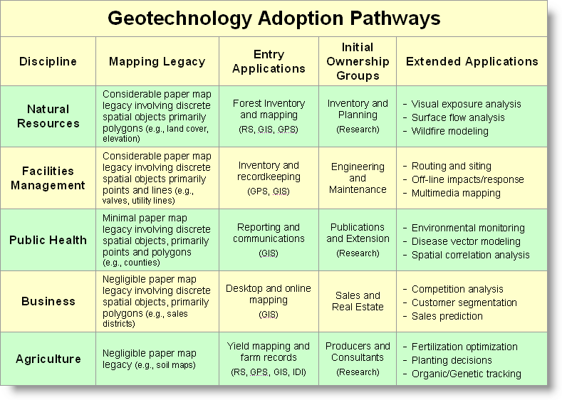
Figure1. Adoption
pathways vary in mapping legacies, early applications and initial ownership groups
to form differing geotechnology paradigms.
The ordering of the list is neither arbitrary nor chronological. It reflects the similarities among mapping legacies, early applications and initial ownership groups that characterize various pathways to GIS. It is interesting to note that while Natural Resources and Agriculture share common sociological, cultural, political and biological footings, their geotechnology adoption paths are radically different, and in fact, form polar extremes.
The Natural Resources community was one of the earliest groups to follow the geographers’ rallying cry in the mid-1970s; enticed by the prospect of automating the mapping process. Their extensive paper-map legacy involved tedious aerial photo interpretation and manual cartography to graphically depict resource inventories over very large areas. The early GIS environment was a natural niche for their well-defined mapping processes and products.
Agriculture, on the other hand had little use for traditional maps, as soil maps are far too generalized and broadly report soil properties instead of nutrient concentrations and other field inputs that farmers manage. Their primary uses for traditional maps were in Boy Scouts or hunting/fishing in mountainous terrain far away from the family farm. This perspective changed in the mid-1990s with the advent of yield mapping that tracks where things are going well and not so good for a crop— a field-level glimpse of the geographic distribution of productivity leading to entirely new site-specific crop management practices.
The alternative perspectives of maps as Images of inventory or as Information for decision-making are the dominant determinants of geotechnology adoption paths. GIS entry was early and committed for those with considerable paper-map legacy and well-defined, easily extended applications. While immensely valuable, automation of traditional applications focus on efficiency, flexibility and cost savings and rarely challenge “how things are done,” or move beyond mapping and basic spatial database management.
Disciplines with minimal paper-map legacies, on the other hand, tend to develop entirely new and innovative applications—the adoption tends to be less evolutionary and more revolutionary. For example, precision agriculture is an application that while barely a decade old, is radically changing crop management practices, as well as guidance and control of farm machinery by extending the traditional spatial triad of RS, GIS and GPS to Intelligent Devices and Implements (IDI) for on-the-fly applications.
The character and constituency of the initial ownership group in a discipline also determines the adoption pathway. For example in the U.S. Forest Service and most Natural Resource entities, the nudge toward GIS was primarily controlled by inventory units at regional and higher bureaucracy levels. The early emphasis of this group was on compiling very large and complex spatial databases over a couple of decades before extensive application of these data—sort of “build it and they (applications) will come.”
Contrast this with the Agriculture ownership group comprised of independent crop consultants and individual farmers focusing on a farm landscape of a few hundred acres per field. The database compilation demands are comparatively minor, and more importantly the return on investment stream must be immediate, not decades. Since they didn’t have a mapping legacy, efficiency and cost saving of data collection/management weren’t the drivers; rather crop productivity and stewardship advancements guided the adoption pathway.
Now turn your attention to the relative positions of the three disciplines in the center of the table. Business’ heritage closely follows that of Agriculture— negligible mapping legacy with radically innovative applications involving a relatively diverse, unstructured and independent user community. Mapping in the traditional sense of “precise placement of physical features” is the farthest thing from the mind of a sales/marketing executive. But a cognitive map that segments a city into different consumer groups, or characterizes travel-time advantages of different stores, or forms a sales prediction surface by product type for a city are fodder for decisions that fully consider spatial information and patterns. From the start, geo-business focused on new ways of doing business and return on investment, not traditional mapping extensions.
Contrast this paradigm with that of a Facilities Management engineer responsible for a transportation district, or an electric transmission network, or an oil pipeline—considerable mapping legacy that exploits basic mapping and spatial database capabilities to better inventory installed assets within a large, structured, utility-based industry. Like Natural Resources, the initial on-the-line mapping entry to GIS is broadening to more advanced applications, such as optimal path routing, off-the-line human/environmental impact analysis and integration of video mapping of assets and surrounding conditions.
Now consider Public Health’s pathway— minimal paper-map legacy primarily for graphic display of aggregated statistics within very large governmental agencies. Its adoption of geotechnology has lagged the other disciplines. This is particularly curious as it has a well-developed and well-funded research component similar to those in Natural Resources and Agriculture. While these units have been proactive in GIS adoption, the heritage of Public Health research is deeply rooted in traditional statistics and non-spatial modeling that has hindered acceptance of advanced spatial statistics and map analysis techniques. The combination of minimal paper-map legacy and minimal enthusiasm for new applications within large bureaucracies has delayed geotechnology adoption in Public Health—a revolution in waiting.
I have used the Geotechnology Adoption Pathways table in numerous workshops and college courses. Invariably, it incites considerable discussion as students ponder their own pathway and extrapolate personal experiences to those of other students and related disciplines. At a minimum, the lively discussion encourages students to think outside their disciplinary box and confirms the multifaceted GIS community that we’ll explore in the next section.
(GeoWorld January, 2007)
While
mapping has been around for thousands of years, its digital expression is only a
few decades old. My first encounter with
a digital map was as an undergrad research assistant in the 1960s with Bob
Colwell’s cutting-edge remote sensing program at UC Berkeley. A grad student had hooked up some
potentiometers to the mechanical drafting arm of a stereographic mapping
device.
The
operator would trace a dot at a constant elevation around the 3D terrain model
of hills and valleys created by a stereo pair of aerial photos. Normally, the mechanical movements of the dot
would drag a pen on a piece of paper to draw a contour line. But the research unit translated the movement
into X, Y coordinates that were fed into a keypunch machine—kawapa, kawapa,
kawapa. After a few months of tinkering,
the “digital contour lines” for the school forest were imprisoned in a couple
of boxes of punch cards.
The
next phase of simply connecting the dots proved the hardest. Although UC Berkeley was a leading research
university with over 42,000 students, there was only one plotter available. And like the Egyptian period there were only
a couple of folks on campus who could write the programming hieroglyphics
needed to control the beast. Heck,
computer science itself was just a fledgling discipline and GIS was barely a
gleam in a few researchers’ eyes.
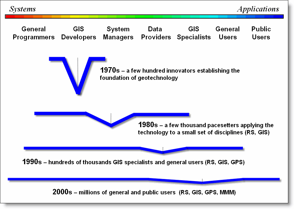
Figure 1. The evolution of the Geotechnology Community
has broadened its membership in numbers, interests, backgrounds and depth of
understanding.
The
old-timer’s story sets the stage for a discussion of the human-ware evolution
in geotechnology (see figure 1). In the
1970s the GIS community consisted of a few hundred research types chipping away
at the foundation. A shared focus of just
getting the technology to work emphasized appropriate data structures, display
capabilities and a few rudimentary operations.
In fact, during this early period a “universal truth” in data structure
was sought that fueled a decade of academic crusades between vector-heads and
raster-heads. My remote sensing
background put me in the dwindling raster camp that eventually circled the
wagons around the pixel (picture element) and image processing that effectively
split GIS and RS for a decade.
The
1980s saw steady growth in GIS and the community expanded from few hundred
researchers to a few thousand pacesetters focused on applying the infant
technology. The community mix enlarged
to include more traditional programmers on the systems side and systems managers,
data providers and GIS specialists in a few of the mapping-oriented
organizations on the application side.
Most of this effort focused on vector processing of discrete spatial
objects (point, line and polygon features).
While the greatest effort was on developing databases, great strides in
cartographic modeling were made to mimic manual map analysis, such as
intersection, overlay, buffer and geo-query.
At the same time, advances in hardware and software began to bring GIS
in reach of more and more organizations; however GIS continued to be a
specialized unit “down the hall and to the right.”
Now
compare the community lines for the 1970s and 1980s in the figure. First note the extension to more professional
experiences—some defining entirely new fields, such as GIS specialist. In addition, the 1980s line flattens a bit to
indicate that the average “depth of expert spatial knowledge” within the
community declined from that of the laser-focused research types. Finally note that the “keel of knowledge”
shifted right toward the system managers and application focus.
These
trends in the GIS community mix accelerated in the 1990s. On the system side professional programmers
restructured, extended and enhanced the old unstructured FORTRAN and BASIC code
of the early innovators into comprehensive flagship GIS systems with graphical
interfaces. The GIS developers stopped
coding their own systems and used the toolkits to develop customized solutions
for individual industries and organizations.
System managers, data providers and GIS specialists provided the utility
and day-to-day attention demanded by the operational systems coming on line.
On the
application side, a maturing GPS industry was fully integrated and RS returned
to the geotechnology fold. As a result,
hundreds of thousands of general users of these systems with varying
backgrounds and application interests found GIS on their desktops and joined
the community mix. The shift toward
applications diminished the depth of knowledge and further shifted its keel to
the right. At one point this prompted me
to suggest that GIS was “a mile wide and an inch deep,” as many in the wave of
new comers to GIS did so through an enlarged job description and a couple of
training courses.
If that
is the case, then we are now ten miles wide and a quarter-inch deep. In retrospect and a bit of reflection on the
2000s community line suggests that is exactly where we should be. While there are large numbers of
deeply-keeled GIS experts, there are orders of magnitude more users of
geotechnology. The evolution from a
research-dominated to a user-dominated field confirms that geotechnology has
come of age. In part, this is a natural
condition of all computer-based disciplines brought on by ubiquitous personal
computers and Internet connections. The
dominant focus of this phase, from webmaster to the end user, is on accessing
spatial information. Couple this with
the current multimedia clamor and 3D visualization, such as Google Earth, a
whole new form of a map is becoming the norm.
So what
is under the flap of the ever enlarging tent of GIS? My guess is that it will become a fabric of
society with most public users not even knowing (or caring) that they are using
geotechnology. At the same time, a growing
number of general users will become more comfortable with the technology and
demand increased capabilities, particularly in spatial analysis, statistics and
modeling.
This
will translate into new demands on developers for schizophrenic systems that are
tiered for various levels of users. Most
users will be satisfied with simply accessing digital forms of traditional
maps, geo-query and driving directions, while other more knowledgeable users,
will access GIS models to run sophisticated map analyses and scenarios for
planning and decision-making.
Also I
suspect that the 2010s will see a whole new community line with two keels like
a catamaran—one on the right (GIS specialist, General Users and Public Users)
emphasizing applications involving millions and another on the left (General
Programmers, GIS Developers and System Managers) emphasizing systems involving
thousands. This dualistic community will
completely change the evolutionary character of the GIS community into a
radically different revolutionary group.
The
biggest challenge we face is educating future GIS professionals and users to
“think with maps” instead of just “mapping.”
The digital nature of modern maps has forever changed what a map is and
how it can be used. Map analysis capabilities
will serve as the catalyst that enables us to fully address cognitive aspects
of geographic space, as well as characterizing discrete physical features.
Innovation
Drives GIS Evolution
(GeoWorld August, 2007)
What I find interesting is that current geospatial
innovation is being driven more and more by users. In the early years of GIS one would dream up
a new spatial widget, code it, and then attempt to explain to others how and why
they ought to use it. This sounds a bit
like the proverbial “cart in front of the horse” but such backward practical
logic is often what moves technology in entirely new directions.
“User-driven innovation,” on the other hand, is in
part an oxymoron, as innovation—“a
creation, a new device or process resulting from study and experimentation”
(Dictionary.com)—is usually thought of as canonic advancements leading
technology and not market-driven solutions following demand. At the moment, the over 500 billion dollar
advertising market with a rapidly growing share in digital media is dominating
attention and the competition for eyeballs is directing geospatial innovation
with a host of new display/visualization capabilities.
User-driven GIS innovation will become more and more
schizophrenic with a growing gap between the two clans of the GIS user
community as shown in figure 1.
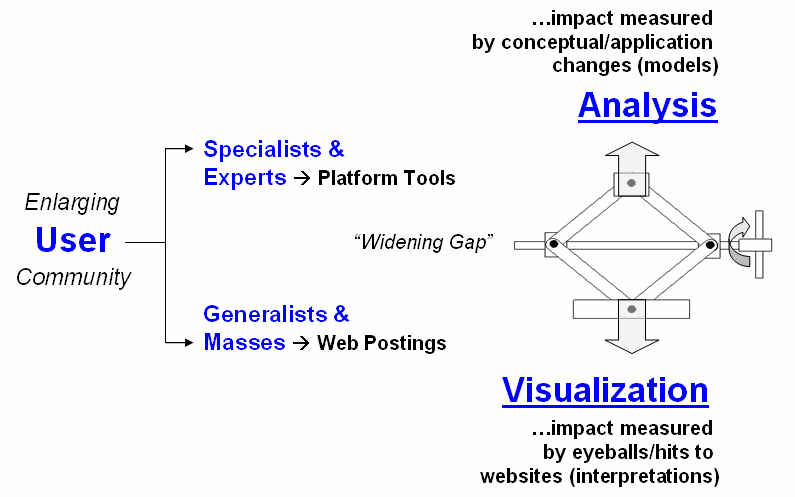
Figure 1. Widening gap in the GIS user community.
Another interesting point is that “radical”
innovation often comes from fields with minimal or no paper map legacy, such as
agriculture and retail sales, because these fields do not have pre-conceived
mapping applications to constrain spatial reasoning and innovation.
In the case of Precision
Agriculture, geospatial technology (GIS/RS/GPS) is coupled with robotics
for “on-the-fly” data collection and prescription application as tractors move
throughout a field. In Geo-business, when you swipe your credit
card an analytic process knows what you bought, where you bought it, where you
live and can combine this information with lifestyle and demographic data
through spatial data mining to derive maps of “propensity to buy” various
products throughout a market area. Keep
in mind that these map analysis applications were non-existent a dozen years
ago but now millions of acres and billions of transactions are part of the
geospatial “stone soup” mix.
As shown in figure 2 the evolution of GIS is more
cyclical than linear. My greybeard
perspective of over 30 years in GIS suggests that we have been here
before. In the 1970s the research and
early applications centered on Computer
Mapping (display focus) that yielded to Spatial
Data Management (data structure/management focus) in the next decade as we
linked digital maps to attribute databases for geo-query. The 1990s centered on GIS Modeling (analysis focus) that laid the groundwork for whole
new ways of assessing spatial patterns and relations, as well as entirely new
applications such as precision agriculture and geo-business.
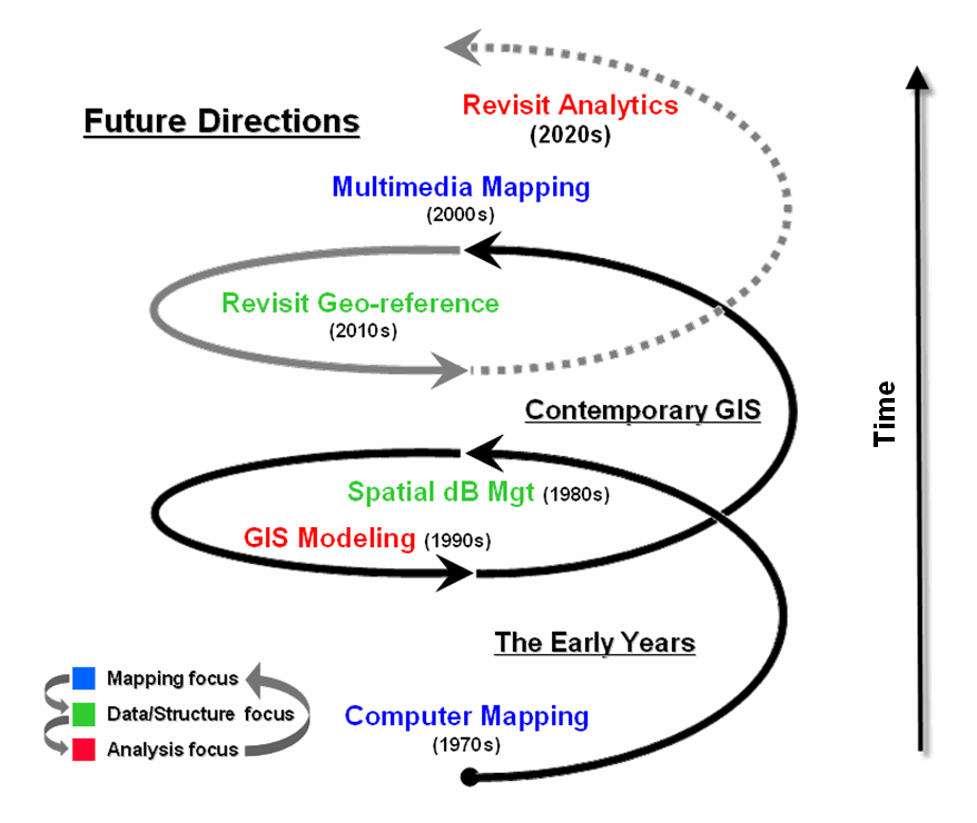
Figure 2. GIS Innovation/Development cycles.
Today, GIS is centered on Multimedia Mapping (mapping focus) which brings us full circle to
our beginnings. While advances in
virtual reality and 3D visualization can “knock-your-socks-off” they represent incremental
progress in visualizing maps that exploit dramatic computer hardware/software
advances. The truly geospatial
innovation awaits the next re-focusing on data/structure and analysis.
The bulk of the current state of geospatial analysis
relies on “static coincidence modeling”
using a stack of geo-registered map layers.
But the frontier of GIS research is shifting focus to “dynamic flows modeling” that tracks
movement over space and time in three-dimensional geographic space. But a wholesale revamping of data structure
is needed to make this leap.
The impact of the next decade’s evolution will be
huge and shake the very core of GIS—the Cartesian coordinate system itself …a spatial
referencing concept introduced by mathematician Rene Descartes 400 years
ago.
The current 2D square for geographic referencing is
fine for “static coincidence” analysis over relatively small land areas, but
woefully lacking for “dynamic 3D flows.”
It is likely that Descartes’ 2D squares will be replaced by hexagons
(like the patches forming a soccer ball) that better represent our curved
earth’s surface …and the 3D cubes replaced by nesting polyhedrals for a
consistent and seamless representation of three-dimensional geographic
space. This change in referencing
extends the current six-sides of a cube for flow modeling to the twelve-sides
(facets) of a polyhedral—radically changing our algorithms as well as our
historical perspective of mapping (see April
2007 Beyond Mapping column for more discussion).
The new geo-referencing framework provides a needed
foothold for solving complex spatial problems, such as intercepting a nuclear
missile using supersonic evasive maneuvers or tracking the air, surface and
groundwater flows and concentrations of a toxic release. While the advanced map analysis applications
coming our way aren’t the bread and butter of mass applications based on
historical map usage (visualization and geo-query of data layers) they
represent natural extensions of geospatial conceptualization and analysis
…built upon an entirely new set analytic tools, geo-referencing framework and a
more realistic paradigm of geographic space.
____________________________
Author’s
Note: I have been
involved in research, teaching, consulting and GIS software development since
1971 and presented my first graduate course in GIS Modeling in 1977. The discussion in these columns is a
distillation of this experience and several keynotes, plenary presentations and
other papers—many are posted online at www.innovativegis.com/basis/basis/cv_berry.htm.
GIS and
the Cloud Computing Conundrum
(GeoWorld September, 2009)
I think my first encounter with the concept of cloud computing
was more than a dozen years ago when tackling a Beyond Mapping column on
object-oriented computing. It dealt with
the new buzzwords of “object-oriented” user interface (OOUI), programming
system (OOPS) and database management (OODBM) that promised to revolutionize
computer interactions and code sets (see Author’s Note). Since then there has been a string of new
evolutionary terms from enterprise GIS, to geography network, interoperability,
distributed computing, web-services, mobile GIS, grid computing and mash-ups
that have captured geotechnology’s imagination, as well as attention.
“Cloud computing” is the latest in this trajectory of
terminology and computing advances that appears to be coalescing these
seemingly disparate evolutionary perspectives.
While my
technical skills are such that I can’t fully address its architecture or
enabling technologies, I might be able to contribute to a basic grasp of what
cloud technology is, some of its advantages/disadvantages and what its
near-term fate might be.
Uncharacteristic
of the Wikipedia, the definition for cloud computing is riddled with
techy-speak, as are most of the blogs.
However, what I am able to decipher is that there are three
distinguishing characteristics defining it (see figure 1)—
1) it
involves virtualized resources …meaning that workloads are allocated
among a multitude of interconnected computers acting as a single device;
2) it
is dynamically scalable …meaning that the system can be readily enlarged;
3) it
acts as a service …meaning that the software and data components are
shared over the Internet.
The
result is a “hosted elsewhere” environment for data and services …meaning that
cloud computing is basically the movement of applications, services, and data
from local storage to a dispersed set of servers and datacenters— an
advantageous environment for many data heavy and computationally demanding
applications, such as geotechnology.
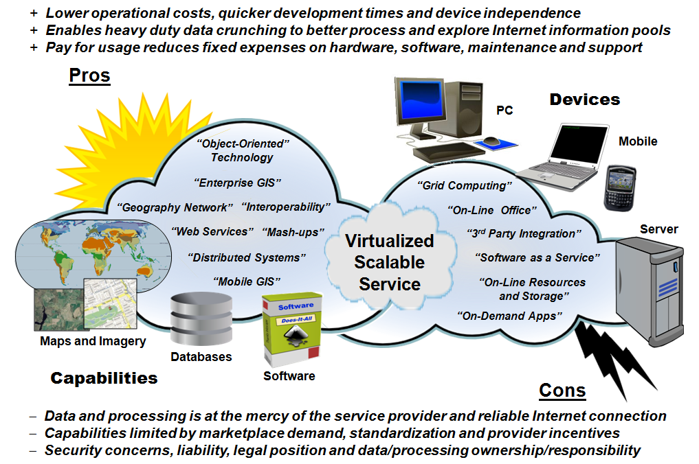
Figure 1. Cloud Computing
characteristics, components and considerations.
A
counterpoint is that the “elsewhere” conjures up visions of the old dumb
terminals of the 70’s connected to an all powerful computer center serving the
masses. It suggests that some of the
tailoring and flexibility of the “personal” part of the PC environment might be
lost to ubiquitous services primarily designed to capture millions of
eyeballs. The middle ground is that
desktop and cloud computing can coexist but that suggests duel markets,
investments, support and maintenance.
Either
way, it is important to note that cloud computing is not a technology—it is a
concept. It essentially presents the
idea of distributed computing that has been around for decades. While there is some credence in the argument
that cloud computing is simply an extension of yesterday’s buzzwords, it
ingrains considerable technical advancement.
For example, the cloud offers a huge potential for capitalizing on the
spatial analysis, modeling and simulation functions of a GIS, as well as
tossing gigabytes around with ease …a real step-forward from the earlier
expressions.
There are two broad types of
clouds depending on their application:
1) “Software as a Service” (SaaS) delivering a single application through the browser to a
multitude of customers (e.g., WeoGeo and Safe Software are making
strides in SaaS for geotechnology)— on the customer side, it means minimal
upfront investment in servers or software licensing and on the provider side,
with just one application to maintain, costs are low compared to conventional
hosting; and,
2) “Utility Computing” offering storage and virtual servers
that can be accessed on demand by stitching together memory, I/O, storage, and
computational capacity as a virtualized resource pool available over the
Internet— thus creating a development
environment for new services and usage accounting.
Google Earth is a good example of early-stage, cloud-like
computing. It seamlessly stitches
imagery from numerous datacenters to wrap the globe in a highly interactive 3D
display. It provides a wealth of geography-based
tools from direction finding to posting photos and YouTube videos. More importantly, it has a developer’s
environment (.kml) for controlling the user interface and custom display of
geo-registered map layers. Like the
iPhone, this open access encourages the development of applications and tools
outside the strict confines of dedicated “flagship” software.
But the
cloud’s silver lining has some dark pockets.
There are four very important non-technical aspects to consider in
assessing the future of cloud computing: 1)
liability concerns, 2) information
ownership, sensitivity and privacy issues, 3)
economic and payout considerations, and 4)
legacy impediments.
Liability
concerns
arise from decoupling data and procedures from a single secure computing
infrastructure— What happens if the data is lost or compromised? What if the data and processing are changed
or basically wrong? Who is
responsible? Who cares?
The
closely related issues of ownership, sensitivity and privacy raise
questions like: Who owns the data? Who is it shared with and under what
circumstances? How secure is the
data? Who determines its accuracy,
viability and obsolescence? Who defines
what data is sensitive? What is personal
information? What is privacy? These lofty questions rival Socrates sitting
on the steps of the Acropolis and asking …what is beauty? …what is truth? But these social questions need to be
addressed if the cloud technology promise ever makes it down to earth.
In
addition, a practical reality needs an economic and payout
component. While SaaS is usually
subscription based, the alchemy of spinning gold from “free” cyberspace straw
continues to mystify me. It appears that
the very big boys like Google and Virtual (Bing) Earths can do it through
eyeball counts, but what happens to smaller data, software and service providers
that make their livelihood from what could become ubiquitous? What is their incentive? How would a cloud computing marketplace be
structured? How will its transactions be
recorded and indemnified?
Governments,
non-profits and open source consortiums, on the other hand, see tremendous
opportunities in serving-up gigabytes of data and analysis functionality for
free. Their perspective focuses on
improved access and capabilities, primarily financed through cost savings. But are they able to justify large
transitional investments to retool under our current economic times?
All
these considerations, however, pale in light legacy impediments, such as
the inherent resistance to change and inertia derived from vested systems and
cultures. The old adage “don’t fix it, if it ain’t broke” often
delays, if not trumps, adoption of new technology. Turning the oil tanker of GIS might take a
lot longer than technical considerations suggest—so don’t expect GIS to
“disappear” into the clouds just yet.
But the future possibility is hanging overhead.
_____________________________
Author’s Note: see online book Map Analysis, Topic 1,
Object-Oriented Technology and Its
Visualizing a
Three-dimensional Reality
(GeoWorld October, 2009)
I have always thought of
geography in three-dimensions. Growing
up in California’s high Sierras I was surrounded by peaks and valleys. The pop-up view in a pair of aerial photos
got me hooked as an undergrad in forestry at UC Berkeley during the 1960’s
while dodging tear gas canisters.
My doctoral work involved a
three-dimensional computer model that simulated solar radiation in a vegetation
canopy (SRVC). The mathematics would
track a burst of light as it careened through the atmosphere and then bounce
around in a wheat field or forest with probability functions determining what
portion was absorbed, transmitted or reflected based on plant material and leaf
angles. Solid geometry and statistics
were the enabling forces, and after thousands of stochastic interactions, the
model would report the spectral signature characteristics a satellite likely
would see. All this was in anticipation
of civilian remote sensing systems like the Earth Resources Technology
Satellite (ERTS, 1973), the precursor to the Landsat program.
This experience further
entrenched my view of geography as three-dimensional. However, the ensuing decades of GIS
technology have focused on the traditional “pancake perspective” that flatten
all of the interesting details into force-fitted plane geometry. Even more disheartening is the assumption
that everything can be generalized into a finite set of hard boundaries
identifying discrete spatial objects defined by points, lines and
polygons. While this approach has served
us well for thousands of years and we have avoided sailing off the edge of the
earth, geotechnology is taking us “where no mapper
has gone before,” at least not without a digital map and a fairly hefty
computer.
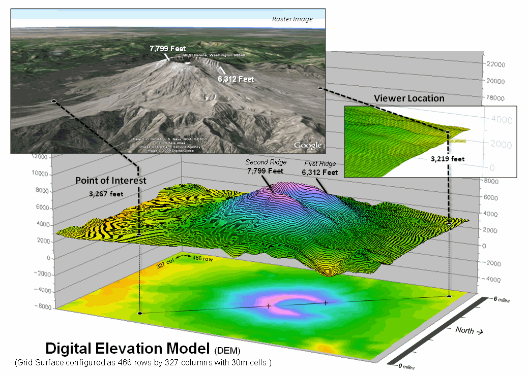
Figure
1. Mount St. Helens topography.
Consider
the Google Earth image of Mount St. Helens in the upper-left portion of figure
1. The peaks poke-up and the valleys dip
down with a realistic land cover wrapper.
This three-dimensional rendering of geography is a far cry from the
traditional flat map with pastel colors imparting an abstract impression of the
area. You can zoom-in and out, spin
around and even fly through the landscape or gaze skyward to the stars and other
galaxies.
Underlying
all this is a Digital Elevation Model (DEM) that encapsulates the topographic
undulations. It uses traditional X and Y
coordinates to position a location plus a Z coordinate to establish its
relative height above a reference geode (sea level in this case). However from a purist’s perspective there are
a couple of things that keep it from being a true three-dimensional GIS. First, the raster image is just that— a
display in which thousands the “dumb” dots coalesce to form a picture in your
mind, not an “intelligent” three-dimensional data structure that a computer can
understand. Secondly, the rendering is
still somewhat two-dimensional as the mapped information is simply “draped” on
a wrinkled terrain surface and not stored in a true three-dimensional GIS—a
warped pancake.
The
DEM in the background forms Mt St. Helen’s three-dimensional terrain surface by
storing elevation values in a matrix of 30 meter grid cells of 466 rows by 327
columns (152, 382 values). In this form,
the computer can “see” the terrain and perform its map-ematical magic.
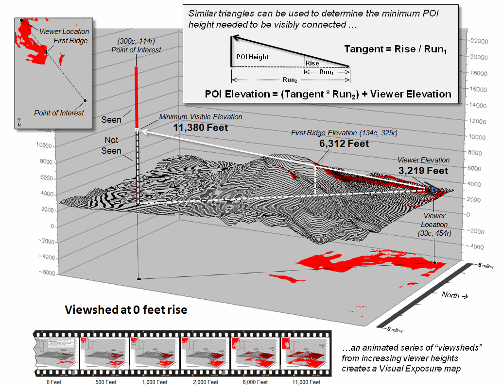
Figure
2. Basic geometric relationships
determine the minimum visible height considering intervening ridges.
Figure
2 depicts a bit of computational gymnastics involving three-dimensional
geography. Assume you are standing at
the viewer location and looking to the southeast in the direction of the point
of interest. Your elevation is 3,219
feet with the mountain’s western rim towering above you at 6,312 feet and
blocking your view of anything beyond it.
In a sense, the computer “sees” the same thing—except in mathematical
terms. Using similar triangles, it can calculate the minimum point-of-interest height
needed to be visibly connected as (see author’s notes for a link to discussion
of the more robust “splash algorithm” for establishing visual connectivity)…
Tangent = Rise / Run
=
(6312 ft – 3219 ft) / (SQRT[(134 – 33)2 + (454 – 325) 2 ]
* 98.4251 ft)
=
3093 ft / (163.835 * 98.4251 ft) = 3893 ft / 16125 ft = 0.1918
Height = (Tangent * Run) + Viewer Height
=
(0.1918 * (SQRT[(300 – 33)2 +
(454 – 114) 2 ] * 98.4251 ft)) + 3219 ft
=
(0.1918 * 432.307 * 98.4251 ft) + 3219 = 11,380 Feet
Since
the computer knows that the elevation on the grid surface at that location is
only 3,267 feet it knows you can’t see the location. But if a plane was flying 11,380 feet over
the point it would be visible and the computer would know it.
Figure
3. 3-D Grid Data Structure is a direct expansion of the 2D structure with X, Y and Z coordinates
defining the position in a 3-dimensional data matrix plus a value
representing the characteristic or condition (attribute) associated with that
location.
Conversely,
if you “helicoptered-up” 11,000 feet (to 14,219 feet elevation) you could see
over both of the caldron’s ridges and be visually connected to the surface at
the point of interest (figure 3). Or in
a military context, an enemy combatant at that location would have
line-of-sight detection.
As
your vertical rise increases from the terrain surface, more and more terrain
comes into view (see author’s notes
for a link to an animated slide set).
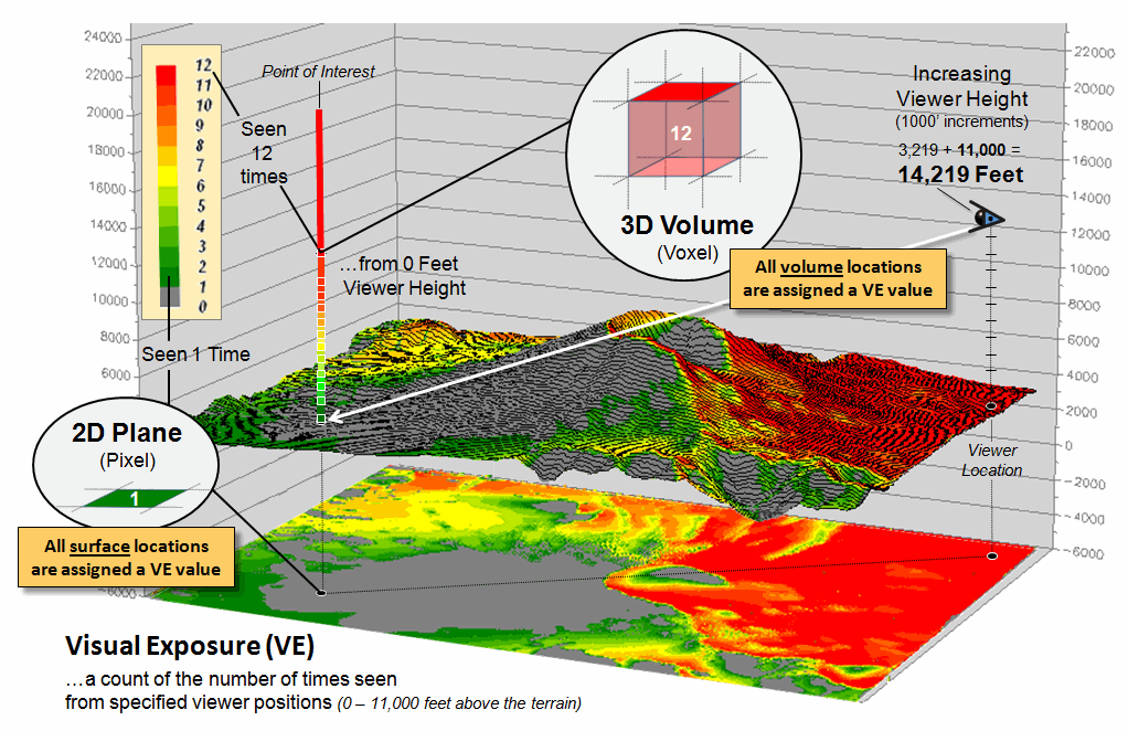
The visual exposure surface draped on the terrain and projected on the
floor of the plot keeps track of the number of visual connections at every grid
surface location in 1000 foot rise increments.
The result is a traditional two-dimensional map of visual exposure at each
surface location with warmer tones representing considerable visual exposure
during your helicopter’s rise.
However,
the vertical bar in figure 3 depicts the radical change that is taking us
beyond mapping. In this case the
two-dimensional grid “cell” (termed a pixel) is replace by a three-dimensional
grid “cube” (termed a voxel)—an extension from the concept of an area on a
surface to a glob in a volume. The
warmer colors in the column identify volumetric locations with considerable
visual exposure.
Now
imagine a continuous set of columns rising above and below the terrain that
forms a three-dimensional project extent—a block instead of an area. How is the block defined and stored; what new
analytical tools are available in a volumetric GIS; what new information is
generated; how might you use it? …that’s fodder for the next section. For me, it’s a blast from the past that is
defining the future of geotechnology.
____________________________
Author’s
Notes: for a more detailed
discussion of visual connectivity see the online book Beyond Mapping III,
Topic 15, “Deriving
and Using Visual Exposure Maps” at www.innovativegis.com/basis/MapAnalysis/Topic15/Topic15.htm. An
annotated slide set demonstrating visual connectivity from increasing viewer
heights is posted at www.innovativegis.com/basis/MapAnalysis/Topic27/AnimatedVE.ppt.
Thinking
Outside the Box (pun intended)
(GeoWorld November, 2009)
Last section used a progressive series of line-of-sight connectivity
examples to demonstrate thinking beyond a 2-D map world to a three-dimensional
world. Since the introduction of the
digital map, mapping geographic space has moved well beyond its traditional
planimetric pancake perspective that flattens a curved earth onto a sheet of
paper.
A
contemporary Google Earth display provides an interactive 3-D image of the
globe that you can fly through, zoom-up and down, tilt and turn much like Luke
Skywalker’s bombing run on the Death Star.
However both the traditional 2-D map and virtual reality’s 3-D
visualization view the earth as a surface—flattened to a pancake or curved and
wrinkled a bit to reflect the topography.
Figure
1 summarizes the key elements in locating yourself on the earth’s surface …sort
of a pop-quiz from those foggy days of Geography 101. The Prime Meridian and Equator serve as base
references for establishing the angular movements expressed in degrees of
Longitude (X) and Latitude (Y) of an imaginary vector from the center of the
earth passing through any location. The
Height (Z) of the vector positions the point on the earth’s surface.
It’s
the determination of height that causes most of us to trip over our geodesic
mental block. First, the globe is not a
perfect sphere but is a squished ellipsoid that is scrunched at the poles and
pushed out along the equator like love-handles.
Another way to conceptualize the physical shape of the surface is to
imagine blowing up a giant balloon such that it “best fits” the actual shape of
the earth (termed the geoid) most often aligning with mean sea level. The result is a smooth geometric equation
characterizing the general shape of the earth’s surface.
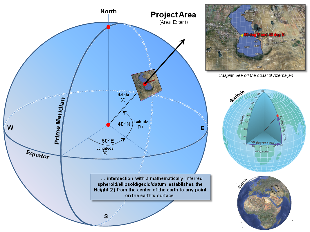
Figure 1. A 3-dimensional coordinate
system uses angular measurements (X,Y) and length (Z) to locate points on the
earth’s surface.
But the earth’s mountains bump-up and valleys bump-down
from the ellipsoid so a datum is designed to fit the earth's
surface that accounts for the actual wrinkling of the globe as established by
orbiting satellites. The most common datum for the world is WGS 84 (World
Geodetic System 1984) used by all GPS
equipment and tends to have and accuracy of +/- 30 meters or less from the
actual local elevation anywhere on the surface.
The
final step in traditional mapping is to flatten the curved and wrinkled surface
to a planimetric projection and plot it on a piece of paper or display on a
computer’s screen. It is at this stage
all but the most fervent would-be geographers drop the course, or at least drop
their attention span.
However,
a true 3-D GIS simply places the surface in volumetric grid elements along with
others above and below the surface. The
right side of figure 2 shows a Project Block containing a million grid elements
(termed “voxels”) positioned by their geographic coordinates—X (easting), Y
(northing) and Z (height). The left side
depicts stripping off one row of the elevation values defining the terrain
surface and illustrating a small portion of them in the matrix by shading the
top’s of the grids containing the surface.
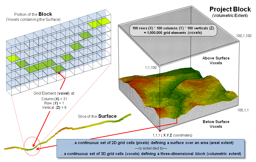
Figure 2. An implied 3-D matrix defines
a volumetric Project Block, a concept analogous to areal extent in traditional
mapping.
At
first the representation in a true 3-D data structure seems trivial and inefficient
(silly?) but its implications are huge.
While topographic relief is stable (unless there is another Mount St.
Helens blow that redefines local elevation) there are numerous map variables
that can move about in the project block.
For example, consider the weather “map” on the evening news that starts
out in space and then dives down under the rain clouds. Or the National Geographic show that shows
the Roman Coliseum from above then
crashes through the walls to view the staircases and then proceeds through the
arena’s floor to the gladiators’ hypogeum with its subterranean
network of tunnels and cages.
Some “real cartographers” might argue that those aren’t
maps but just flashy graphics and architectural drawings …that there has been a
train wreck among mapping, computer-aided drawing, animation and computer
games. On the other hand, there are
those who advocate that these disciplines are converging on a single view of
space—both imaginary and geographic. If
the X, Y and Z coordinates represent geographic space, nothing says that Super
Mario couldn’t hop around your neighborhood or that a car is stolen from your
garage in Grand Theft Auto and race around the streets in your hometown.
The
unifying concept is a “Project Block” composed of millions of
spatially-referenced voxels.
Line-of-sight connectivity determines what is seen as you peek around a
corner or hover-up in a helicopter over a mountain. While the mathematics aren’t for the
faint-hearted or tinker-toy computers of the past, the concept of a “volumetric
map” as an extension of the traditional planimetric map is easy to grasp—a
bunch of three-dimensional cubic grid elements extending up and down from our
current raster set of squares (bottom of figure 3).
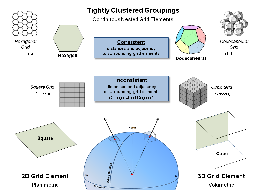
Figure 3. The hexagon and dodecahedral are alternative
grid elements with consistent nesting geometry.
However,
akin to the seemingly byzantine details in planimetric mapping, things aren’t
that simple. Like the big bang of the
universe, geographic space expands from the center of the earth and a simple
stacking of fixed cubes like wooden blocks won’t align without significant
gaps. In addition, the geometry of a cube
does not have a consistent distance to all of its surrounding grid elements and
of its twenty six neighbors only six share a complete side with the remaining
neighbors sharing just a line or a single point. This inconsistent geometry makes a cube a poor
grid element for 3-D data storage.
Similarly,
it suggests that the traditional “square” of the Cartesian grid is a bit
limited—only four complete sides (orthogonal elements) and four point
adjacencies (diagonal). Also, the
distances to surrounding elements are different (a ratio of 1:1.414). However, a 2D hexagon shape (beehive honey
comb) abuts completely without gaps in planimetric space (termed “fully
nested”); as does a combination of pentagon and hexagon shapes nests to form
the surface of a spheroid (soccer ball).
To help
envision an alternative 3-D grid element shape (top-right of figure 3) it is
helpful to recall Buckminster Fuller's book Synergetics and his classic treatise of various
"close-packing" arrangements for a group of spheres. Except in this instance, the sphere-shaped
grid elements are replaced by "pentagonal dodecahedrons"— a set of
uniform solid shapes with 12 pentagonal faces (termed geometric “facets”) that
when packed abut completely without gaps (termed fully “nested”).
All of
the facets are identical, as are the distances between the centroids of the
adjoining clustered elements defining a very “natural” building block (see
Author’s Note). But as always, “the
Devil is in the details” and that discussion is dealt with in the next
section.
_____________________________
Author’s Note: In 2003, a team of cosmologists and
mathematicians used NASA’s WMAP cosmic background radiation data to develop a
model for the shape of the universe. The
study analyzed a variety of different shapes for the universe, including finite
versus infinite, flat, negatively- curved (saddle-shaped), positively- curved
(spherical) space and a torus (cylindrical). The study revealed that the
math adds up if the universe is finite and shaped like a pentagonal
dodecahedron (http://physicsworld.com/cws/article/news/18368). And
if one connects all the points in one of the pentagon facets, a
5-pointed star is formed. The ratios of the lengths of the resulting line
segments of the star are all based on phi, Φ, or 1.618… which is the
“Golden Number” mentioned in the Da Vinci Code as the universal constant of
design and appears in the proportions of many things in nature from DNA to the human
body and the solar system—isn’t mathematics wonderful!
From a
Mapping Pancake to a Soufflé
(GeoWorld November, 2009)
As the Time Traveller
noted in H. G. Wells’ classic “The Time Machine,” the real world has
three geometric dimensions not simply the two we commonly use in mapping. In fact, he further suggested that “...any
real body must have extension in four directions: Length, Breadth, Thickness—and
Duration (time)” …but that’s a whole other story.
Recall from last
section’s discussion of 3D GIS that Geodetic Referencing (geographic
position) used in identifying an “areal extent” in two-dimensions on the
earth’s surface can be extended to a Database Referencing system (matrix
location) effectively defining a 3-dimensional “project block” (see the left
side of figure 1). The key is the use of
Geodetic Height above and below the earth’s ellipsoid as measured along
the perpendicular from the ellipsoid to provide the vertical (Z) axis for any
location in 3-dimensional space.
The result is a
coordinate system of columns (X), rows (Y), and verticals (Z) defining an
imaginary matrix of grid elements, or “voxels,” that are a direct conceptual
extension of the “pixels” in a 2D raster image. For example, the top-right inset in figure 1
shows a 3D map of a cave system using ArcGIS 3D Analyst software. The X, Y and Z positioning forms a
3-dimensional display of the network of interconnecting subterranean
passages. The lower-right inset shows an
analogous network of blood vessels for the human body except at much different
scale. The important point is that both
renderings are 3D visualizations and not a 3D GIS as they are unable to
perform volumetric analyzes, such as directional flows along the passageways.
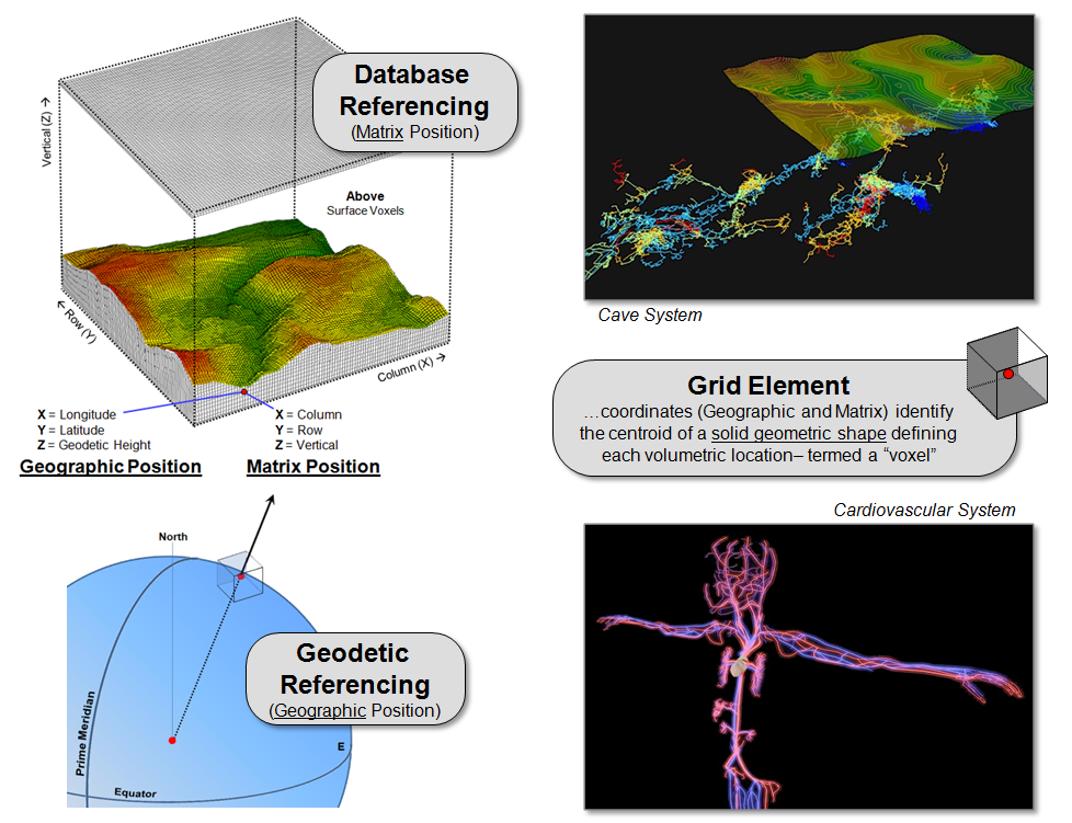
Figure 1. Storage of a vertical (Z) coordinate extends
traditional 2D mapping to
3D volumetric
representation.
The distinction between
3D visualization and analytical systems arises from differences in their data
structures. A 3D visualization system
stores just three values—X and Y for “where” and Z for “what (elevation).” A 3-dimensional mapping system stores at least
four values—X, Y and Z for “where” and an attribute value for “what” describing
the characteristic/condition at each location within a project block.
Figure 2 illustrates two ways of storing
3-dimensional grid data. A Flat File stores a single map value for
each grid element in a map block. The
individual records can explicitly identify each grid element (grayed
columns—“where”) along with the attribute (black column—“what”). Or, much more efficiently, the information
can be implicitly organized as a header line containing the grid block
configuration/size/referencing followed by a long string of numbers with each
value’s position in the string determining its location in the block through
standard nested programming loops. This
shortened format provides for advanced compression techniques similar to those
used in image files to greatly reduce file size.
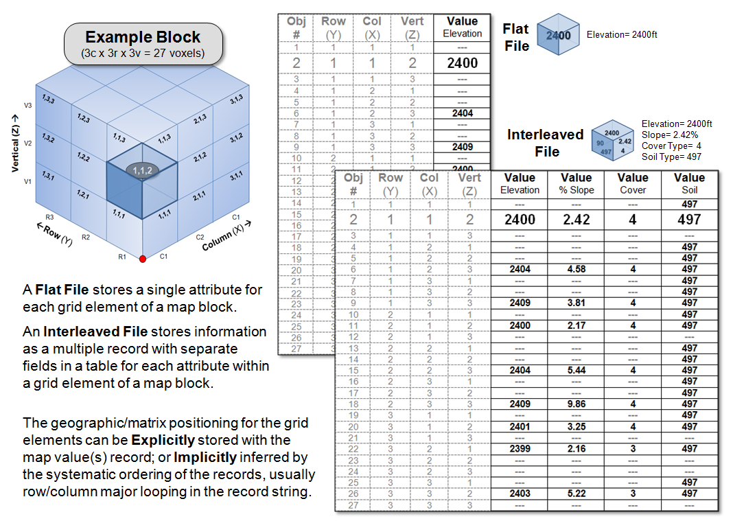
Figure 2. A 3-dimensional matrix structure can be used
to organize volumetric mapped data.
An alternative strategy, termed an Interleaved File, stores a series of map
attributes as separate fields for each record that in turn represents each grid
element, either implicitly or explicitly organized into a table. Note that in the interleaved file in figure
2, the map values for Elevation, %Slope and Cover type identify surface
characteristics with a “null value (---)” assigned to grid elements both above
and below the surface. Soil type, on the
other hand, contains values for the grid elements on and immediately below the
surface with null values only assigned to locations above ground. This format reduces the number of files in a
data set but complicates compression and has high table maintenance overhead
for adding and deleting maps.
Figure 3 outlines some broader issues and future
directions in 3D GIS data storage and processing. The top portion suggests that the
inconsistent geometry of the traditional Cube
results in differing distances and facet adjacency relationship to the
surrounding twenty six neighbors, thereby making a cube a poor grid element for
3D data storage. A Dodecahedron, on the other hand, aligns with a consistent set of 12
equidistant pentagonal faces that “nest” without gaps ...an important condition
in spatial analysis of movements, flows and proximal conditions.
The lower portion of figure 3 illustrates the knurly
reality of geographic referencing in 3-dimensions—things change as distance
from the center of the earth or bounding ellipsoid changes. Nicely nesting grid elements of a fixed size
separate as distance increases (diverge); overlap as distance decreases
(converge). To maintain a
“close-packing” arrangement either the size of the grid element needs to adjust
or the progressive errors of fixed size zones are tolerated.
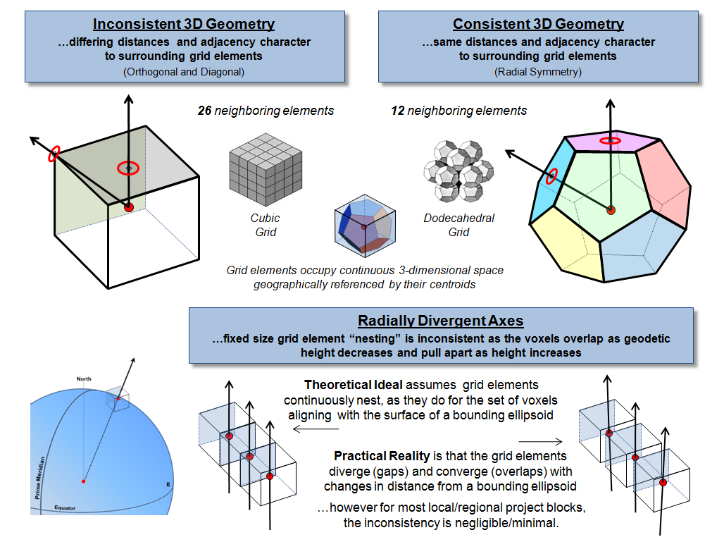
Figure 3. Alternative grid element shapes and new
procedures for dealing with radial divergence form the basis for continued 3D
GIS research and development.
Similar historical changes in mapping paradigms and
procedures occurred when we moved from a flat earth perspective to a round
earth one that generated a lot of room for rethinking. There are likely some soon-to-be-famous
mathematicians and geographers who will match the likes of Claudius Ptolemy
(90-170), Gerardus Mercator (1512-1594) and Rene Descartes (1596-1650)— I wonder who among us will take us beyond mapping
as we know it?
_____________________________
Author’s Notes: A good discussion of polyhedral and other 3-dimensional coordinate
systems is in Topic 12, “Modeling locational uncertainty via hierarchical tessellation,”
by Geoffrey Dutton in Accuracy of Spatial Databases edited by Goodchild
and Gopal. In his discussion he notes
that “One common objection to polyhedral data models for GIS is that
computations on the sphere are quite cumbersome … and for many applications the
spherical/geographical coordinates … must be converted to and from Cartesian
coordinates for input and output.”
(Back to the Table of Contents)