Beyond Mapping III
|
Map
Analysis book with companion CD-ROM for hands-on exercises and further reading |
Extending GIS
Procedures with Variable-Width Buffers — discusses
the basic considerations in establishing variable-width buffers that respond to
both intervening conditions and the type of connectivity
Line-of-Sight Buffers Add Intelligent to Maps — describes
procedures for creating buffers that track relative visual exposure and noise
levels
Create Effective Distance Buffers to Improve
Map Accuracy — develops
procedures for creating buffers that respond to the relative ease of
movement
Author’s
Notes: The figures in this topic use MapCalcTM
software. An educational CD with online
text, exercises and databases for “hands-on” experience in these and other
grid-based analysis procedures is available for US$21.95 plus shipping and
handling (www.farmgis.com/products/software/mapcalc/
).
<Click here> right-click to download a
printer-friendly version of this topic (.pdf).
(Back to the Table of Contents)
______________________________
Extending
(GeoWorld,
November 2000, pg. 24-25)
In part, the graphical and inventory aspects of traditional maps have dominated the digital translation of spatial information. Users can enter an address and instantly view a map of that location and print a set of driving instructions. One can publish a couple of hundred scanned topographic sheets on a CD that can be panned and zoomed at several scales. Images and even streaming video can be linked to their precise locations on a map and accessed over the web simply by clicking on an embedded symbol.
The digital expression of familiar mapping procedures
represented the first wave in recasting
A good example of infusing extended
Most folks immediately recognize the shortcomings of a simple buffer. Common sense tells us that while delineating a single “as-the-crow-flies” distance under all possible intervening conditions might meet the letter of the law, it often violates reality. The concept of variable-width buffers that match reality has been with us for years—what is missing is a traditional mindset and experience with a tool. What is needed for second wave applications is education that fosters understanding and confidence in the extended procedures.
|
|
|
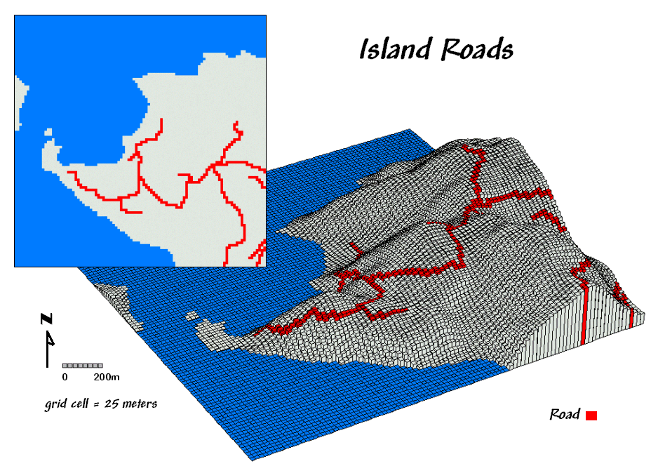
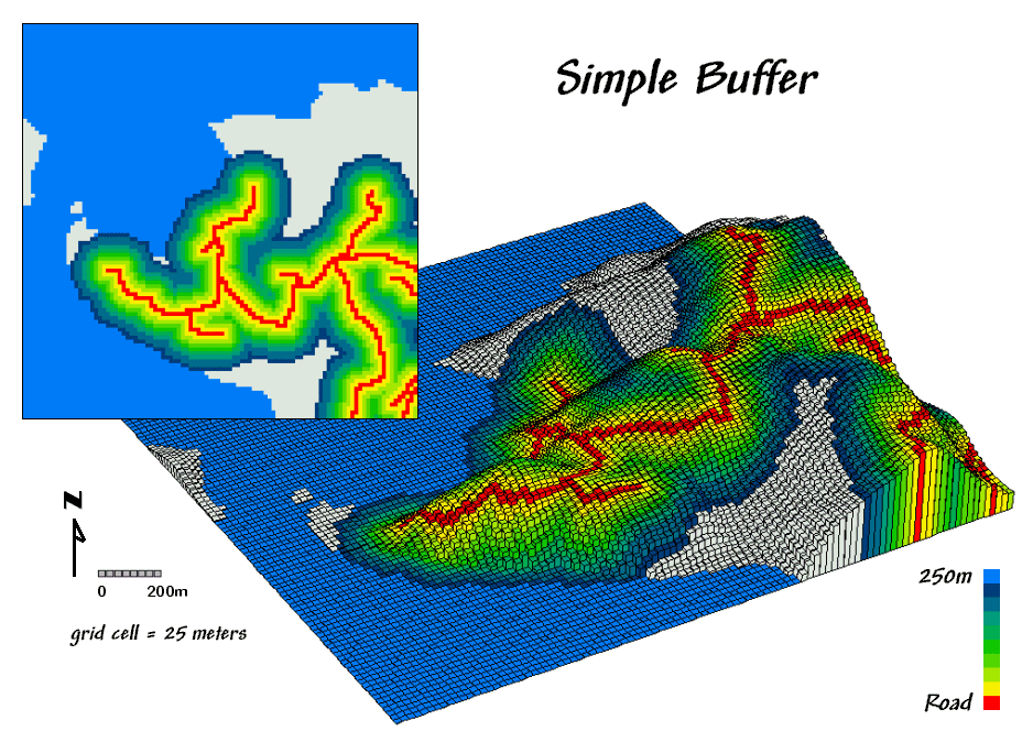
Figure 1. A Simple Proximity Buffer identifies the
distance to roads throughout the buffered area.
Note that the buffer extends into the ocean—an inappropriate “reach” for
terrestrial applications.
Consider the road network and its 250-meter Simple Proximity Buffer as depicted in figure 1. In most desktop mapping systems a “Buffer Tool” is used to automatically inscribe a line at a given distance from a complex feature. The dark blue edge of the buffer in the figure identifies this maximum reach. However, the color progression indicates the relative proximity within the buffer—from yellow (close) to dark blue (far). While most folks have little experience with a simple proximity buffer, they immediately relate to the concept and value of the added information.
Also they immediately see some of its limitations. Notice how the consistent reach causes the buffer to extend into unintended areas—the ocean in this case. The “geographic slop” is more than graphically troublesome, it can skew statistics and misrepresent spatial relationships for terrestrial applications.
|
|
|
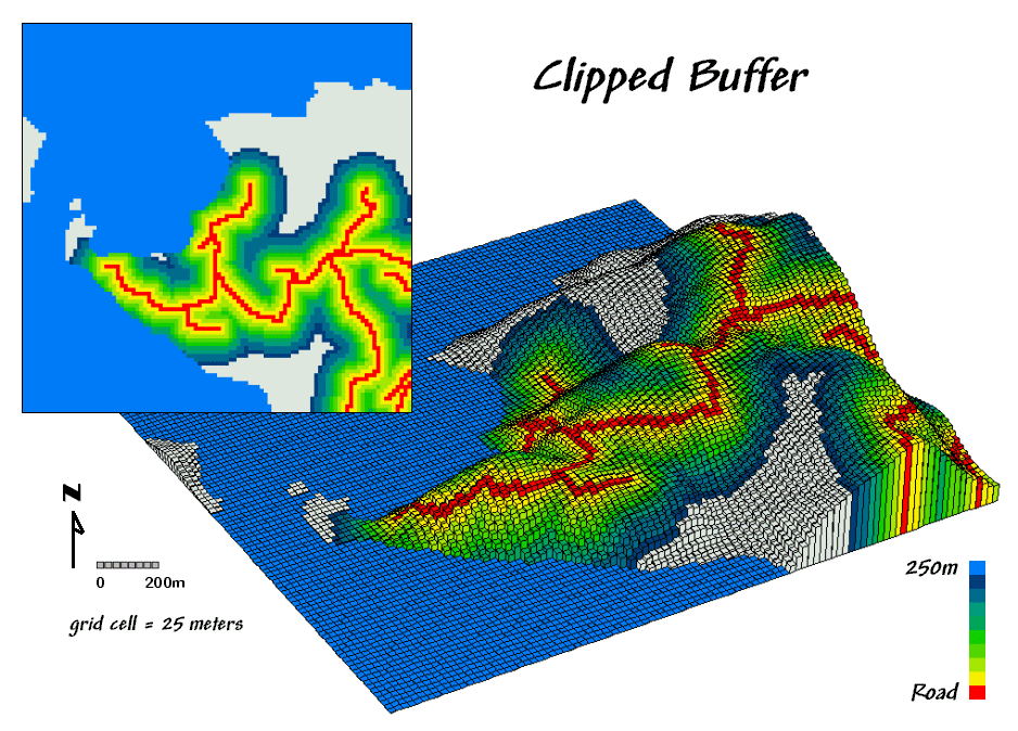
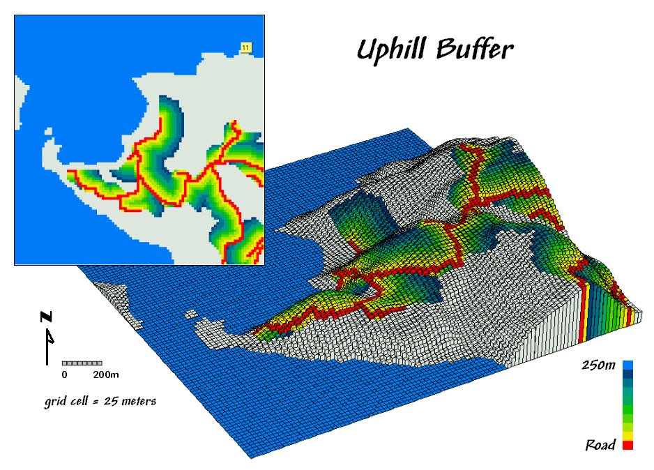
Figure 2. The figure on the left clips the simple buffer to represent only land areas. The figure on the right uses the elevation surface to identify only areas that are uphill from the roads.
The left side of figure 2 shows a Clipped Buffer,
the first conceptual step toward variable-width buffers. Some
For example, consider the Uphill Buffer maps on the right side of figure 2. In this instance the measurement of proximity for the buffered area was forced to extend only “uphill” from the roads as defined on a guiding surface (a short conceptual step from a masking map). The results draped over the elevation surface confirms that only uphill locations are identified. By simply specifying “downhill” only those locations that are below the roads (and not within in the ocean mask) would be identified.
The division of a simple buffer into its uphill and downhill components can be important. A road engineer sees different land slippage considerations in the two areas. An environmental scientist concentrates on the downhill portion for flows of oil and other chemicals from the road. In fact in most applications consideration of the characteristics and conditions within a buffer are at least as important as the outline of its extent.
The ability to establish proximity-based buffers that react to geographic conditions isn’t part of our paper map legacy. However, the concept is ingrained in practical experience. As subsequent columns in this mini-series will show, the ability to identify up/downwind buffers, noise attenuation buffers, customer travel-time buffers and other effective proximity buffers that respond to geographic conditions are no longer beyond our reach. The tools are at hand (and actually have been for quite sometime). What awaits is a second wave of innovative applications that take advantage of the new tools and instill their commonplace acceptance.
Line-of-Sight Buffers Add
Intelligent to Maps
(GeoWorld,
December 2000, pg. 24-25)
As noted in the previous section, simple buffers are often just that—too simple for real world applications. The assumption that there are uniform conditions throughout a fixed distance from a map feature rarely squares with reality. A consistent 100, 200 or 300-meter buffer around roads often includes inappropriate results within a buffer, such as ocean areas. Or they can include areas that are inconsistent with an assumption, such as a concern for just the uphill locations from roads.
Variable-width buffers, on the other hand, respond to both intervening conditions and the type of connectivity. They expand and contract to reflect spatial reality around map features by clipping inappropriate and inconsistent areas.
Tracking the variations within a buffer is just as important. Instead of simply being within or outside a buffered area, each location can be identified as to its proximity to the buffered feature. For example, all of the uphill locations within 250 meters (variable-width buffer) can be assigned their proximity to a road—a continuum of information throughout the buffer instead of simply an “in or out” characterization.
Another type of variable-width buffer involves line-of-sight connectivity. In this application a viewer location “looks” over an elevation surface up to a specified distance and identifies all of the areas it can see.
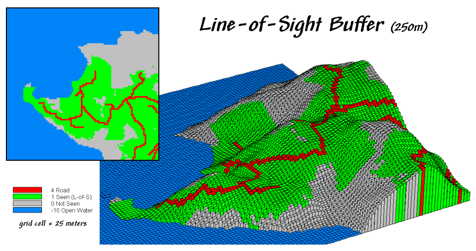
Figure 1.
The “viewshed” of the road network forms a variable-width, line-of-sight
buffer.
Figure 1 shows a 250-meter line-of-sight buffer surrounding the road network. Note that variations in the terrain cause the buffer to truncate areas that are not seen, yet are still within the 250-meter reach.
The conceptual basis for calculating line-of-sight connectivity is quite simple. The position of a viewer location (one of the road cells in this example) determines its height from an elevation map of the area. The cell’s height is compared to the elevations of its eight surrounding cells to establish a set of rise-to-run ratios—change in elevation per horizontal distance. The rise/run ratios for the next ring of cells are computed. If a new location’s ratio is greater, it is marked as seen and its ratio becomes the one to beat for subsequent locations in that direction. The process is repeated for successive rings up to the buffer limit. Then the next viewer cell is considered until the entire road network has been evaluated.
In practice, the line-of-sight procedure is a bit more complex as additional factors, such as vegetation height, often are included in determining the viewshed defining the buffered area. Also, the process can be extended to keep track of the number of times each buffer location is seen (e.g., number of road cells connected to it). The result is a measure of visual exposure for each buffer location. Instead of simply delineating the buffer limits, information about the relative exposure throughout the buffer is noted.
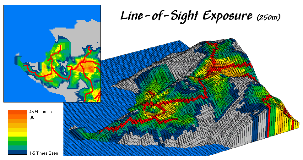
Figure 2. A
“visual exposure” map identifies the number of times each map location is
visually connected to an extended map feature.
Figure 2 contains a map of the visual exposure within the 250-meter viewshed. Note the four areas of relatively high exposure to roads (warmer tones). While these areas might be ideal for visually aesthetic activities, the areas of minimal exposure (cool tones) or those entirely outside the buffer (gray) are more suitable for “ugly things.” For example, a national park might use a visual exposure buffer to assist forest planning for foreground management zones. A telecom company might use the information to help locate cell-towers.
Or a developer might focus on candidate areas for “Soothing Acres Estates” that have minimal visual exposure and road noise. Spatial modeling of noise dissipation can be a complex undertaking, but line-of-sight connectivity is a fundamental element. While sound waves bend more than light waves, they also tend to be blocked by intervening terrain. A road on the other side of a ridge is neither seen nor heard—provided there is a big pile of dirt separating the source and receptor.
Also, sound waves fade dramatically as a function of distance (1/d2). Figure 3 incorporates this dissipation for a line-of-sight noise buffer. The cells adjacent to the road are the loudest (yellow—1.00 times the noise level). Those at the limit of the 250-meter reach are a whole lot quieter (blue—0.010 times the noise level). Noise levels at cells that have intervening terrain or are beyond the buffer-reach (gray) are considered inaudible.
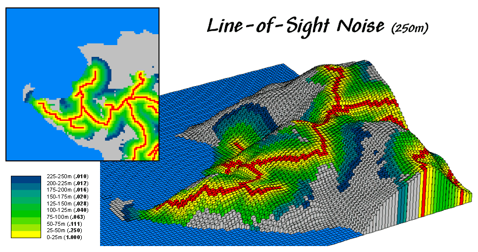
Figure3. A “noise buffer” considers distance as well
as line-of-sight connectivity.
Admittedly, the assumptions in modeling noise dissipation in
this example are simplified, but they do reflect reality better than a simple
buffer that totally ignores the very real effects of distance and surrounding
terrain. There are several possibilities
for improving the accuracy of the noise levels within the buffer, such as
treating neighboring vegetation types differently. However, these extensions involve
consideration of “relative barriers” in characterizing variable-width
buffers—the topic for next month’s column.
_______________________
Author's Note: for a complete discussion of noise
analysis and abatement, see www.nonoise.org/library/highway/policy.htm.
Create Effective Distance
Buffers to Improve Map Accuracy
(GeoWorld, January 2001, pg. 24-25)
One of the most fundamental operations in
Figure 1, on the other hand, shows some of the extensions to traditional buffering that were discussed in the past couple of columns. Inset a) characterizes the relative proximity of all locations within a road buffer of 250 meters. Inset b) clips the road buffer for infeasible areas, such as open water. A buffer identifying just the uphill areas from the road is shown in inset c). Insets d) and e) characterize the locations within 250 meters that can be seen from the road network (Viewshed) and their relative amount of visual exposure (Expose).
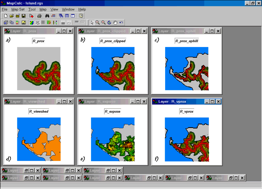
Figure 1.
Examples of Variable-Width and Line-of-Sight Buffers.
Inset f) shows the proximity to the road for areas within the viewshed buffer. This information can be useful in determining visual impact—locations that are seen a lot and are near roads equate to high visual impact. Similarly, noise dissipation can be coarsely modeled as inversely related to line-of-sight distance—it’s fairly quiet at locations that are relatively near the road but on the other side of a ridge (outside the line-of-sight buffer).
The previous discussions should have you rethinking the utility of scribing lines that are “everywhere-the-same” in characterizing the influences about a map feature. In the real world, spatial context is rarely as simple as implied by the lines of a traditional buffer.
For example, consider hiking in mountainous terrain. In gentle terrain you move along at a brisk pace. But as the terrain becomes steeper, progress slows until eventually there are slopes that repels most hikers (no pun intended). It is common sense that steep intervening conditions can make locations “effectively” farther away. Conversely, gentle intervening slopes make locations much more accessible.
The effect of slope on defining a buffer’s reach is developed in Figure 2. The top left inset is a map of the slope conditions from 0 to 100 percent. The Hiking_Friction map calibrates the slopes in terms of the relative ease of foot-travel— 0-5% Easy, 5-10% Moderate, 10-20% Hard, 20-40% Difficult, and >40% a no-go situation.
It is important to note that the value 1 is assigned to the easiest conditions to cross and all other slope conditions are assigned a value indicating increased difficulty— 2= twice as hard, 5= five times as hard, 10= ten times as hard and –2 for inaccessible no-go areas.
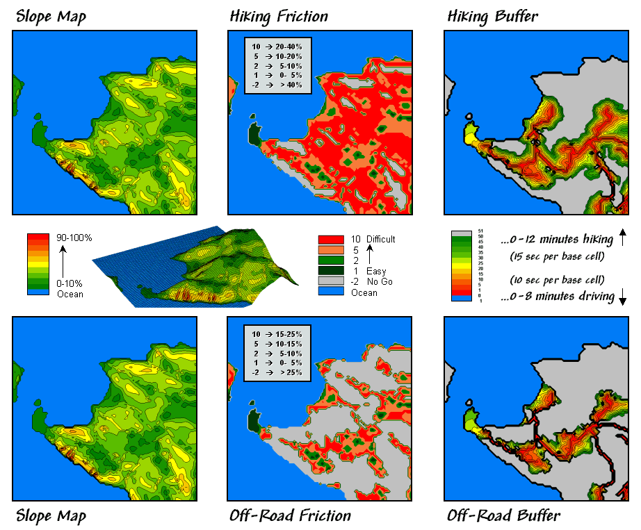
Figure 2.
Development of Effective-Distance Buffers for Hiking and off-road
travel.
Calibration of these values relate to the relative “cost” of traversing a grid cell and in this instance it was assumed to take 15 seconds to cross the easiest 25 meter cell. A moderate cell, on the other hand, is twice as difficult and takes 30 seconds to cross; a hard cell takes 75 seconds (1.25 minutes); and a difficult cell takes 250 seconds (4.17 minutes). An effective-distance operation is used that extends and contacts the width of the buffer considering the intervening conditions as calibrated on the friction map (Hiking_Buffer inset in figure 2).
In this instance, an effective buffer reach of 50 cells was used. If the road were surrounded completely by gentle slopes, the buffer would extend a consistent 50 cells from all locations and have the appearance of a traditional buffer. However, as steeper areas are encountered the geographic reach is shortened. In fact the portion of the road in the lower right of the map is surrounded by “no-go” conditions and the buffer is truncated at the edge of the road.
The lower set of maps in figure 2 repeats the analysis to create an effective-distance buffer assuming vehicular off-road travel. The slope map was calibrated for off-road travel assuming an 10 second base friction for the gentle slopes (0-5%); 20 seconds for 5-10%; 50 seconds for 10-15%; 100 seconds (1.7 minutes) for 15-25%; and >25% a no-go situation. Note the extensive area of inaccessible regions identified in the Off-Road_Friction map giving the buffer a spindly look.
Now compare the hiking and off-road buffers based on effective-distance. A significantly larger portion of the Off-Road_Buffer is classified as inaccessible. An effective reach of 50 cells is used in both cases, but the calibration generates a 0 to 12 minute buffer for hiking and a 0 to 8 minute buffer for an off-road vehicle. In both instances, the effective buffers are radically different from that of a traditional fixed-width buffer and provide considerable more information about relative movement within the buffered area.
Figure 3 literally extends the processing a bit farther by increasing the reach to encompass all accessible areas by hiking or off-road travel. The blue tones on each map identify incrementally larger reaches beyond the buffers shown in figure 2. Note that the areas reached by off-road travel is significantly less than those reached by hiking.
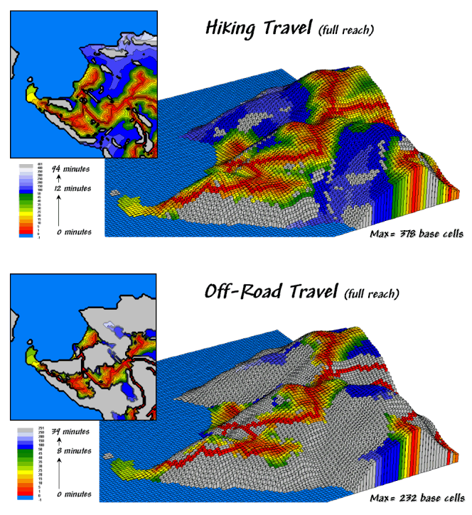
Figure 3.
Comprehensive Travel-Time Maps for Hiking and Off-Road Movement.
Also note the extended reach shown for the area in the lower right portion of project. The off-road travel map extends along a relatively gentle ridge but stops abruptly as the slopes exceed 25%. The hiking travel map, on the other hand, extends along the ridge and clear to the ocean. The gray tones indicate areas that are beyond reach (inaccessible) and can occur as pockets. The farthest location for a hiker is 94 minutes (378 effective cells) and for a off-road vehicle, is 39 minutes (232 effective cells).
One’s first encounter with variable-width buffers might seem a bit uncomfortable since we can’t create them with a ruler, but the concept aligns with common sense. A traditional buffer makes the broad assumption that the reach is everywhere the same. The different types of variable-width buffers reject this assumption and attempt to characterize the intervening conditions and their affects on the buffer’s reach.
Of course the accuracy of the new buffers depends on the exactness of the ancillary data and the algorithms underlying the enabling map analysis operations. However, in most applications the inherent inaccuracy of the underlying assumption of traditional buffers far outweighs these concerns—a simple buffer is most often simply wrong.
____________________
(Back to the Table of
Contents)